Prody Basics
This tutorial aims to teach basic data structures and functions in ProDy.
First, we need to import required packages:
from prody import *
from numpy import *
from matplotlib.pyplot import *
%matplotlib inline
confProDy(auto_show=False)
confProDy(auto_secondary=True)
These import commands will load numpy, matplotlib, and ProDy into the memory. confProDy is used to modify the default behaviors of ProDy. Here we turned off auto_show so that the plots can be made in the same figure, and we turn on auto_secondary to parse the secondary structure information whenever we load a PDB into ProDy. See here for a complete list of behaviors that can be changed by this function. This function only needs to be called once, and the setting will be remembered by ProDy.
Loading PDB files and visualization
ProDy comes with many functions that can be used to fetch data from Protein Data Bank.
The standard way to do this is with parsePDB, which will download a PDB file if needed and load it into a variable of a special data type called an AtomGroup:
p38 = parsePDB('1p38')
p38
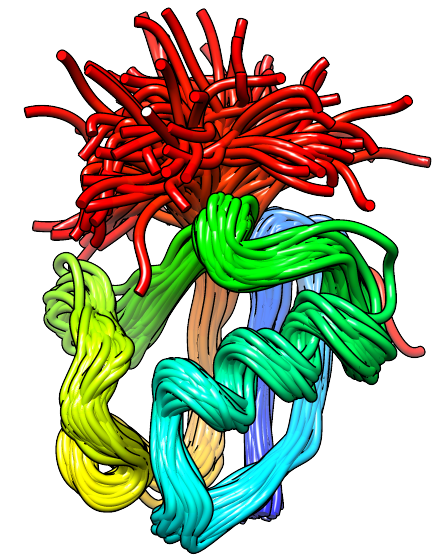
To visualize the structure, we do the following:
showProtein(p38);
legend();

If you would like to display the 3D structure using other packages or your own code, you can get the 3D coordinates via the getCoords method, which returns a NumPy ndarray:
coords = p38.getCoords()
coords.shape
We can also visualise the contact map as follows:
showContactMap(p38.ca);

An AtomGroup is essentially a collection of protein atoms. Each atom can be indexed/queried/found by the following way:
p38[10]
This will give you the $11^{th}$ atom from p38, noting that Python index starts from 0. We can also examine the spatial location of this atom by querying the coordinates, which we can also use to highlight this atom in a plot.
p38[10].getCoords()
showProtein(p38);
ax3d = gca()
x, y, z = p38[10].getCoords()
ax3d.plot([x], [y], [z], 'bo', markersize=20);

We could select a chain, e.g. chain A, of the protein by indexing using its identifier, as follows:
p38['A']
p38['A'].getSequence()
In many cases, it is more convenient to examine the structure with residue numbers, and AtomGroup supports indexing with a chain ID and a residue number:
p38[10].getResnum()
p38['A', 5]
This will give you the residue with the residue number of atom 10, which is an arginine in p38. Please note the difference between this line and the previous one.
p38['A', 5].getNames()
Note that some ProDy objects may not support indexing using a chain identifier or a residue number. In such cases, we can first obtain a hierarchical view of the object:
hv = p38.getHierView()
And then use HierView to index with a chain identifier and residue number as it will always be supported:
hv['A', 5]
Retrieving data from an AtomGroup
Many properties of the protein can be acquired by functions named like "getxxx". For instance, we can obtain the B-factors by:
betas = p38.getBetas()
betas.shape
In this way, we can obtain the B-factor for every single atom. However, in some cases, we only need to know the B-factors of alpha-carbons. We have a shortcut for this:
p38.ca
betas = p38.ca.getBetas()
betas.shape
plot(betas);
ylabel('B-factor');
xlabel('Residue index');

If we would like to use residue numbers in the PDB, instead of the indices as the x-axis of the plot, it would be much more convenient to use the ProDy plotting function, showAtomicLines.
showAtomicLines(betas, atoms=p38.ca);
ylabel('B-factor');
xlabel('Residue number');

We can also obtain the secondary structure information as an array:
p38.ca.getSecstrs()
To make it easier to read, we can convert the array into a string using the Python's built-in function, join :
''.join(p38.ca.getSecstrs())
C is for coil, H for alpha helix, I for pi helix, G for 3-10 helix, and E for beta strand (sheet).
To get a complete list of "get" functions, you can type p38.get<TAB>. We provide a cell for doing this here:
p38
The measure module contains various additional functions for calculations for structural properties. For example, you can calculate the phi angle of the 11th residue:
calcPhi(p38['A', 10])
Note that the residue at the N-terminus or C-terminus does not have a Phi or Psi angle, respectively.
If we calculate the Phi and Psi angle for every non-terminal residue, we can obtain a Ramachandran plot for a protein. An example of Ramachandran plot for human PCNA is shown below:
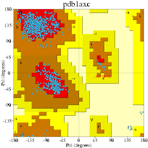
Three favored regions are shown in red -- upper left: beta sheet; center left: alpha helix; center right: left-handed helix. Each blue data point corresponds to the two dihedrals of a residue. We will reproduce this plot for ubiquitin (only the points).
chain = p38['A']
Phi = []; Psi = []; c = []
for res in chain.iterResidues():
    try:
        phi = calcPhi(res)
        psi = calcPsi(res)
    except:
        continue
    else:
        Phi.append(phi)
        Psi.append(psi)
        if res.getResname() == 'GLY':
            c.append('black')
        else:
            secstr = res.getSecstrs()[0]
            if secstr == 'H':
                c.append('red')
            elif secstr == 'G':
                c.append('darkred')
            elif secstr == 'E':
                c.append('blue')
            else:
                c.append('grey')
In the above code, we use an exception handler to exclude the terminal residues from the calculation.
scatter(Phi, Psi, c=c, s=10);
xlabel('Phi (degree)');
ylabel('Psi (degree)');

Selection
In theory you could retrieve any set of atoms by indexing the AtomGroup, but it would be cumbersome to do so. To make it more convienient, ProDy provides VMD-like syntax for selecting atoms. Here lists a few common selection strings. For a more complete tutorial on selection, please see here.
ca = p38.select('calpha')
ca
bb = p38.select('backbone')
bb
We could also perform some simple selections right when the structure is being parsed. For example, we can specify that we would like to obtain only alpha-carbons of chain A of p38 as follows:
chainA_ca = parsePDB('1p38', chain='A', subset='ca')
We could find the chain A using selection (as an alternative to the indexing method shown above):
chA = p38.select('calpha and chain A')
chA
Selection also works for finding a single residue or multiple residues:
res = p38.ca.select('chain A and resnum 10')
res.getResnums()
res = p38.ca.select('chain A and resnum 10 11 12')
res.getResnums()
head = p38.ca.select('resnum < 50')
head.numAtoms()
We can also select a range of residues as follows:
fragment = p38.ca.select('resnum 50 to 100')
If we have data associated to the full length of the protein, we can slice the data using the sliceAtomicData:
subbetas = sliceAtomicData(betas, atoms=p38.ca, select=fragment)
We can visualize the data of this range using showAtomicLines:
showAtomicLines(subbetas, atoms=fragment);
xlabel('Residue number');
ylabel('B factor');

Or highlight the subset in the plot of the whole protein:
showAtomicLines(betas, atoms=p38.ca, overlay=True);
showAtomicLines(subbetas, atoms=fragment, overlay=True);
xlabel('Residue number');
ylabel('B factor');

Selection also allows us to extract particular amino acid types:
args = p38.ca.select('resname ARG')
args
Again, combined with sliceAtomicData and showAtomicLines, we can highlight these residues in the plot of the whole protein:
argbetas = sliceAtomicData(betas, atoms=p38.ca, select=args)
showAtomicLines(betas, atoms=p38.ca, overlay=True);
showAtomicLines(argbetas, atoms=args, linespec='r*', overlay=True);

argbetas = sliceAtomicData(betas, atoms=p38.ca, select=args)
showAtomicLines(betas, atoms=p38.ca, overlay=True);
showAtomicLines(argbetas, atoms=args, linespec='r*', overlay=True);
xlabel('Residue number');
ylabel('B factor');

Compare and align structures
You can also compare different structures using some of the methods in proteins module. Let’s parse another p38 MAP kinase structure.
bound = parsePDB('1zz2')
You can find similar chains in structure 1p38 and 1zz2 using the matchChains function
results = matchChains(p38, bound)
results[0]
In Python, a tuple (or any indexable objects) can be unpacked as follows:
apo_chA, bnd_chA, seqid, overlap = results[0]
The first two terms are the mapping of the proteins to each other,
apo_chA
bnd_chA
the third term is the sequence identity,
seqid
and the forth term is the sequence coverage or overlap:
overlap
If we calculate RMSD right now, we will obtain the value for the unsuperposed proteins:
calcRMSD(bnd_chA, apo_chA)
showProtein(bnd_chA);
showProtein(apo_chA);
legend();

After superposition, the RMSD will be much improved,
bnd_chA, transformation = superpose(bnd_chA, apo_chA)
calcRMSD(bnd_chA, apo_chA)
showProtein(bnd_chA);
showProtein(apo_chA);
legend();

We can also visualize the superposition of the full proteins as the transform matrix is applied to the entire structure:
showProtein(p38);
showProtein(bound);
legend();

Advanced Visualization
Using matplotlib, we only obtained a very simple linear representation of proteins. ProDy also supports a more sophisticated way of visualizing proteins in 3D via py3Dmol:
import py3Dmol
showProtein(p38)
The limitation is that py3Dmol only works in an iPython notebook. You can always write out the protein to a PDB file and visualize it in an external program:
writePDB('bound_aligned.pdb', bnd_chA)