Calculations

Here are the required imports again. You do not need to repeat them if you are still in the same python session.

In [1]: from prody import *

In [2]: from pylab import *

In [3]: ion()

Loading the structure and running adaptive ANM

First, we parse the structures that we want to analyse with Adaptive ANM. For this tutorial, we will use chain A of PDB structures 1GRU and 1GR5, which correspond to the R’’ and T states, which we will call r and t.

We load the structures with only calpha atoms, which we use in downstream steps.

In [4]: r = parsePDB('1gruA', subset='ca')

In [5]: t = parsePDB('1gr5A', subset='ca')

In order to have the same number of atoms in both structures, we use the function alignChains() to create AtomMap objects with the same number.

As r has more atoms (524) than t (517), we provide t first to find the common atoms that are present in t:

In [6]: tmap = alignChains(t, r)[0]

This new implementation of Adaptive ANM increases the number of modes calculated each cycle depending on which ones were used in the previous cycles and their overlaps. We can give it keyword arguments for the maximum number of modes to use (3N-6 by default for N atoms), starting number of modes (20 by default), and other ANM parameters. These parameters can also be presented to the functions below.

Next, we can run AdaptiveANM calculations simply by

In [7]: ens = calcAdaptiveANM(r, tmap, 20)

In [8]: ens
Out[8]: <Ensemble: 1gruA_ca_aANM (32 conformations; 524 atoms)>

The implementation in ProDy also provides 3 ways of running calculations, namely, AANM_ALTERNATING, AANM_ONEWAY, and AANM_BOTHWAYS. AANM_ALTERNATING updates r and tmap simultaneously as in the original Adaptive ANM ([ZY09]) with minor variations, whereas AANM_ONEWAY and AANM_BOTHWAYS carry out the calculations from either just one or both directions (starting with A and going until convergence then continuing from B). This behavior is controlled by the mode argument:

In [9]: ens_1w = calcAdaptiveANM(r, tmap, 20, mode=AANM_ONEWAY)

Analysis

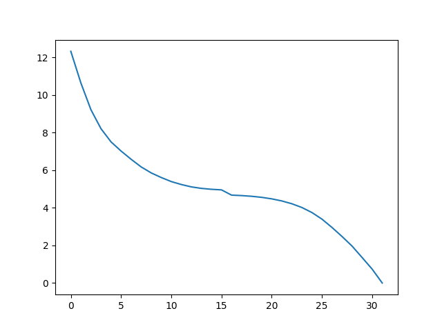
calcAdaptiveANM() creates an Ensemble object that has all the generated, intermediate conformations that bridges r and tmap. The reference coordinates of ens are set to those of tmap, so that we can verify the result by checking the RMSDs of the conformations:

In [10]: plot(ens.getRMSDs())
Out[10]: [<matplotlib.lines.Line2D at 0x7f844c4de2d0>]

In [11]: xlabel('R -> T')
Out[11]: Text(0.5,23.5222,'R -> T')

In [12]: ylabel('RMSD')
Out[12]: Text(47.0972,0.5,'RMSD')

We can also perform any other analysis that is applicable to a Ensemble: object. Other quantities that may be useful for debugging or validation purposes can be obtained through assigning a callback function. For example, to extract the number of modes used in each iteration, we can write the following function to access and store the value:

In [13]: N_MODES = []

In [14]: def callback(**kwargs):
   ....:    modes = kwargs.pop('modes')
   ....:    N_MODES.append(len(modes))
   ....: 

Note that N_MODES needs to be defined outside the function, at a global scope, in order to save the value for each iteration. modes is a ModeSet object that gives you the mode(s) selected for deform the structure in an iteration. You have the access to all the properties of modes, and therefore the whole ANM, but here we are only evaluating the number of selected modes using len(). Please check out the documentation of calcAdaptiveANM() for a complete list of accessible quantities.

Now, we pass the callback function to calcAdaptiveANM() as follows:

In [15]: ens_1w = calcAdaptiveANM(r, tmap, 20, mode=AANM_ONEWAY, callback_func=callback)

And check the number of modes being selected in each iteration:

In [16]: print(N_MODES)
[1, 1, 1, 1, 1, 1, 2, 3, 3, 5, 10, 14, 20, 40, 76, 142, 160, 320, 518, 518]