Calculations

This is the first part of a lengthy example. In this part, we perform the calculations using a p38 MAP kinase (MAPK) structural dataset. This will reproduce the calculations for p38 that were published in [AB09].

We will obtain a PCA instance that stores the covariance matrix and principal modes describing the dominant changes in the dataset. The PCA instance and principal modes (Mode) can be used as input for the functions in dynamics module.

Retrieve dataset

We start by importing everything from the ProDy package:

In [1]: from prody import *

In [2]: from pylab import *

In [3]: ion()

We use a list of PDB identifiers for the structures that we want to include in our analysis.

In [4]: pdbids = ['1P38', '1A9U', '1BL6', '1BL7', '1BMK', '1DI9', '1IAN', '1KV1', '1KV2',
   ...:           '1LEW', '1LEZ', '1M7Q', '1OUK', '1OUY', '1OVE', '1OZ1', '1P38',
   ...:           '1R39', '1R3C', '1W7H', '1W82', '1W83', '1W84', '1WBN', '1WBO',
   ...:           '1WBS', '1WBT', '1WBV', '1WBW', '1WFC', '1YQJ', '1YW2', '1YWR',
   ...:           '1ZYJ', '1ZZ2', '1ZZL', '2BAJ', '2BAK', '2BAL', '2BAQ', '2EWA',
   ...:           '2FSL', '2FSM', '2FSO', '2FST', '2GFS', '2GHL', '2GHM', '2GTM',
   ...:           '2GTN', '2I0H', '2NPQ', '2OKR', '2OZA', '3HVC', '3MH0', '3MH3',
   ...:           '3MH2', '2PUU', '3MGY', '3MH1', '2QD9', '2RG5', '2RG6', '2ZAZ',
   ...:           '2ZB0', '2ZB1', '3BV2', '3BV3', '3BX5', '3C5U', '3L8X', '3CTQ',
   ...:           '3D7Z', '3D83', '2ONL']
   ...: 

Note that we used a list of identifiers that are different from what was listed in the supporting material of [AB09]. Some structures have been refined and their identifiers have been changed by the Protein Data Bank. These changes are reflected in the above list.

Also note that it is possible to update this list to include all of the p38 structures currently available in the PDB using the blastPDB() function as follows:

In [5]: p38_sequence = '''GLVPRGSHMSQERPTFYRQELNKTIWEVPERYQNLSPVGSGAYGSVCAAFDTKTGHRV
   ...: AVKKLSRPFQSIIHAKRTYRELRLLKHMKHENVIGLLDVFTPARSLEEFNDVYLVTHLMGADLNNIVKCQKLTDDH
   ...: VQFLIYQILRGLKYIHSADIIHRDLKPSNLAVNEDCELKILDFGLARHTDDEMTGYVATRWYRAPEIMLNWMHYNQ
   ...: TVDIWSVGCIMAELLTGRTLFPGTDHIDQLKLILRLVGTPGAELLKKISSESARNYIQSLAQMPKMNFANVFIGAN
   ...: PLAVDLLEKMLVLDSDKRITAAQALAHAYFAQYHDPDDEPVADPYDQSFESRDLLIDEWKSLTYDEVISFVPPPLD
   ...: QEEMES'''
   ...: 

To update list of p38 MAPK PDB files, you can make a blast search as follows:

In [6]: blast_record = blastPDB(p38_sequence)

In [7]: pdbids = blast_record.getHits(90, 70)

We use the same set of structures to reproduce the results. After we listed the PDB identifiers, we obtain them using parsePDB() function as follows:

In [8]: structures = parsePDB(pdbids, subset='ca', compressed=False)

The structures variable contains a list of AtomGroup instances.

Prepare ensemble

X-ray structural ensembles are heterogenenous, i.e. different structures have different sets of unresolved residues. Hence, it is not straightforward to analyzed them as it would be for NMR models (see NMR Models). However, ProDy has a function buildPDBEnsemble() that makes this process a lot easier. It depends on mapping each structure against the reference structure using a function such as mapOntoChain() demonstrated in the BLAST example. The reference structure is automatically the first member of list provided, which in this case is 1p38.

In [9]: ensemble = buildPDBEnsemble(structures, title='p38 X-ray')

In [10]: ensemble
Out[10]: <PDBEnsemble: p38 X-ray (78 conformations; 351 atoms)>

Perform an iterative superimposition:

In [11]: ensemble.iterpose()

Save coordinates

We use PDBEnsemble to store coordinates of the X-ray structures. The PDBEnsemble instances do not store any other atomic data. If we want to write aligned coordinates into a file, we need to pass the coordinates to an AtomGroup instance. Then we use writePDB() function to save coordinates:

In [12]: writePDB('p38_xray_ensemble.pdb', ensemble)
Out[12]: 'p38_xray_ensemble.pdb'

PCA calculations

Once the coordinate data are prepared, it is straightforward to perform the PCA calculations:

In [13]: pca = PCA('p38 xray')           # Instantiate a PCA instance

In [14]: pca.buildCovariance(ensemble)   # Build covariance for the ensemble

In [15]: pca.calcModes()                 # Calculate modes (20 of the by default)

Approximate method

In the following we are using singular value decomposition for faster and more memory efficient calculation of principal modes:

In [16]: pca_svd = PCA('p38 svd')

In [17]: pca_svd.performSVD(ensemble)

The resulting eigenvalues and eigenvectors may show differences due to missing atoms in the datasets:

In [18]: abs(pca_svd.getEigvals()[:20] - pca.getEigvals()).max()
Out[18]: 52.62871786506555

In [19]: abs(calcOverlap(pca, pca_svd).diagonal()[:20]).min()
Out[19]: 0.05203202716847314

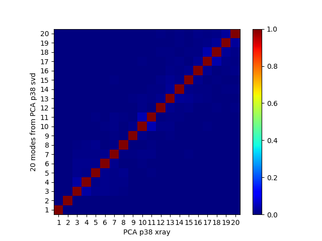
In [20]: showOverlapTable(pca, pca_svd[:20])
Out[20]: 
(<matplotlib.image.AxesImage at 0x7f843e4e1c90>,
 [],
 <matplotlib.colorbar.Colorbar at 0x7f843fe901d0>)

If we remove the most variable loop from the analysis, then these results become much more similar:

In [21]: ref_selection = structures[0].select('resnum 5 to 31 36 to 114 122 to 169 185 to 351')

In [22]: ensemble.setAtoms(ref_selection)

In [23]: pca = PCA('p38 xray')           # Instantiate a PCA instance

In [24]: pca.buildCovariance(ensemble)   # Build covariance for the ensemble

In [25]: pca.calcModes()                 # Calculate modes (20 of the by default)

In [26]: pca_svd = PCA('p38 svd')

In [27]: pca_svd.performSVD(ensemble)

In [28]: abs(pca_svd.getEigvals()[:20] - pca.getEigvals()).max()
Out[28]: 0.4172548564277463

In [29]: abs(calcOverlap(pca, pca_svd).diagonal()[:20]).min()
Out[29]: 0.9986015086878944

In [30]: showOverlapTable(pca, pca_svd[:20]);

Note that building and diagonalizing the covariance matrix is the preferred method for heterogeneous ensembles. For NMR models or MD trajectories, the SVD method may be preferred over the covariance method.

ANM calculations

We also calculate ANM modes for p38 in order to make comparisons later:

In [31]: anm = ANM('1p38')                 # Instantiate a ANM instance

In [32]: anm.buildHessian(ref_selection)   # Build Hessian for the reference chain

In [33]: anm.calcModes()                   # Calculate slowest non-trivial 20 modes

Save your work

Calculated data can be saved in a ProDy internal format to use in a later session or to share it with others.

If you are in an interactive Python session, and wish to continue without leaving your session, you do not need to save the data. Saving data is useful if you want to use it in another session or at a later time, or if you want to share it with others.

In [34]: saveModel(pca)
Out[34]: 'p38_xray.pca.npz'

In [35]: saveModel(anm)
Out[35]: '1p38.anm.npz'

In [36]: saveEnsemble(ensemble)
Out[36]: 'p38_X-ray.ens.npz'

In [37]: writePDB('p38_ref_selection.pdb', ref_selection)
Out[37]: 'p38_ref_selection.pdb'

We use the saveModel() and saveEnsemble() functions to save calculated data. In Analysis, we will use the loadModel() and loadEnsemble() functions to load the data.