Mechanical Stiffness Calculations

This example shows how to perform mechanical resistance calculation for GFP protein (1gfl) and visualize the results using Matplotlib library and VMD program.

An ANM instance that stores Hessian matrix and normal mode data describing the intrinsic dynamics of the protein structure will be used as an input (model) as well as cooridinates of protein structure (coords, pdb).

See [EB08] for more information about the theory of mechanical resistance calculations and more examples.

Parse structure

We start by importing everything from the ProDy package:

In [1]: from prody import *

In [2]: from pylab import *

In [3]: ion()   # turn interactive mode on

We start by parsing chain A of PDB structure 1gfl together with the header, which will be used later for visualizing the secoundary structure.

In [4]: gfp, header = parsePDB('1gflA', header=True)

In [5]: gfp
Out[5]: <AtomGroup: 1gflA (1967 atoms)>

We want to use only Cα atoms for our calculations, so we select them into a new object calphas:

In [6]: calphas = gfp.ca

In [7]: calphas
Out[7]: <Selection: 'ca' from 1gflA (230 atoms)>

Build Hessian and calculate ANM modes

In the next step we instantiate an ANM instance:

In [8]: anm = ANM('GFP ANM analysis')

Then, build the Hessian matrix by passing selected atoms (230 Cα atoms) to ANM.buildHessian() method:

In [9]: anm.buildHessian(calphas, cutoff=13.0)

And calculate all anm modes as they will be needed for later:

In [10]: anm.calcModes(n_modes='all')

All modes are required to perform accurate mechanical stiffness calculations.

Stiffness Matrix Calculations

Mechanical stiffness calculations for the selected group of atoms can be performed using the calcMechStiff() function:

In [11]: stiffness = calcMechStiff(anm, calphas)

In [12]: stiffness
Out[12]: 
array([[0.        , 8.54744466, 8.55133411, ..., 8.73270017, 8.36529536,
        7.42692504],
       [8.54744466, 0.        , 8.89990284, ..., 8.98097054, 8.61849698,
        7.77257692],
       [8.55133411, 8.89990284, 0.        , ..., 8.87863489, 8.55675667,
        7.84521673],
       ...,
       [8.73270017, 8.98097054, 8.87863489, ..., 0.        , 8.87731778,
        8.36590599],
       [8.36529536, 8.61849698, 8.55675667, ..., 8.87731778, 0.        ,
        9.52997339],
       [7.42692504, 7.77257692, 7.84521673, ..., 8.36590599, 9.52997339,
        0.        ]])

To show the stiffness matrix as an image map use the following function:

In [13]: show = showMechStiff(stiffness, calphas, cmap='jet_r')

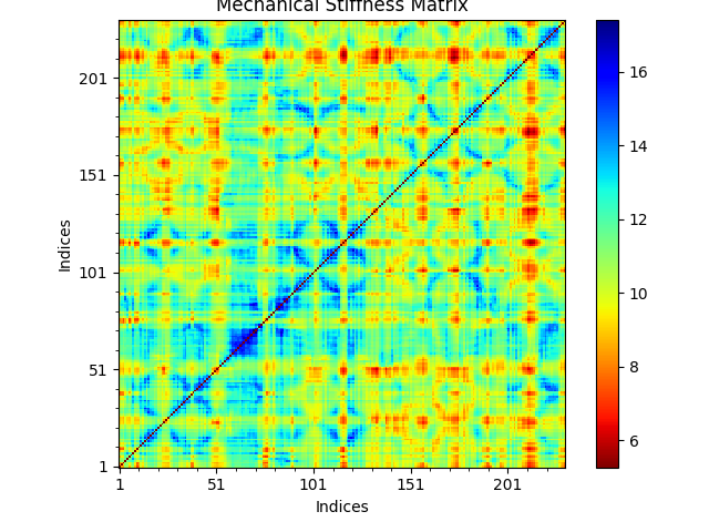
Note that ‘jet_r’ is the reverse of the jet colormap and is similar to the default coloring method of the VMD program.

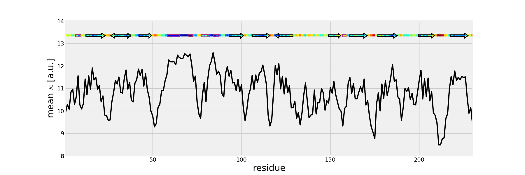
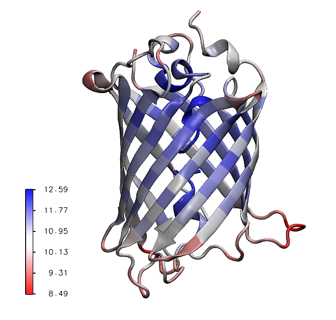
The mean values of the mechanical stiffness matrix for each residue can be calculated using the showMeanMechStiff() function where the secoundary structure of the protein is drawn using header information.

In [14]: show = showMeanMechStiff(stiffness, calphas, header, 'A', cmap='jet_r')

Mechanical Stiffness in VMD

We can generate tcl files for visualizing mechanical stiffness with VMD using the writeVMDstiffness() function. Select one residue in indices ([3]) or series of residues ([3, 7] means from 3 aa to 7 aa inclusive) and a range of effective spring constant k_range ([0, 7.5]).

We provide gfp as well as calphas so VMD has information about the complete protein structure, which it can use for graphical representations.

In [15]: writeVMDstiffness(stiffness, gfp, [3,7], [0,7.5], filename='1gfl_3-7aa')

In [16]: writeVMDstiffness(stiffness, gfp, [3], [0,7], filename='1gfl_3aa')

A TCL file will be saved automatically and can be used later in VMD by running the following command line instruction. Results can be loaded automatically to VMD by setting keyword loadToVMD=True.

:: vmd -e 1gfl_3aa.tcl

or typing the following in the VMD TKConsole (VMD Main) for Linux, Windows and Mac users:

:: play 1gfl_3aa.tcl

The tcl file contains a method for drawing lines between selected pairs of residues, which are highlighted as spheres. The color of the line can be modified by changing the draw color red line in the output file. Only colors from VMD Coloring Method will work. Other changes can be done within VMD in the Graphical Representations menu.

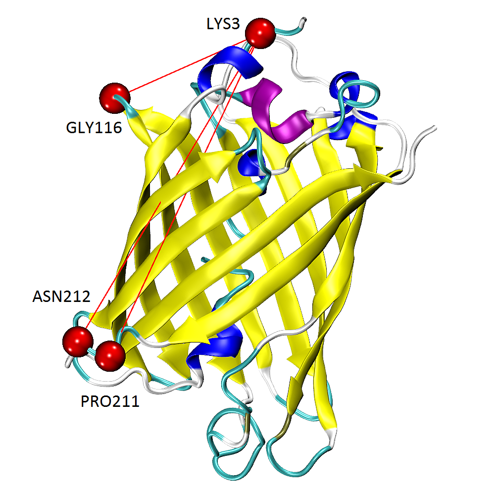
The figure shows GFP results from writeVMDstiffness() function opened in VMD. Pairs of found residues LYS3-GLY116, LYS3-PRO211 and PRO211-ASN212 are shown as VDW spheres connected with red lines.

Additionally, 1gfl_3aa.txt file is created. It contains a list of residue pairs with the value of effective spring constant (in a.u. because kBT=1) obtained from calcMechStiff().

LYS3    GLY116  6.91650667766
LYS3    PRO211  6.85989128668
LYS3    ASN212  6.69507284967
...

The range of spring constant for k_range can be checked as follows:

In [17]: calcStiffnessRange(stiffness)
Out[17]: (5.271418245781293, 17.384909446532433)

See also calcMechStiffStatistic() and calcStiffnessRangeSel() functions for more detailed analysis of the stiffness matrix.

The results of the mean value of mechanical stiffness calculation can be seen in VMD using:

In [18]: writeDeformProfile(stiffness, gfp, select='chain A and name CA', pdb_selstr='protein')

Calculate Distribution of Deformation

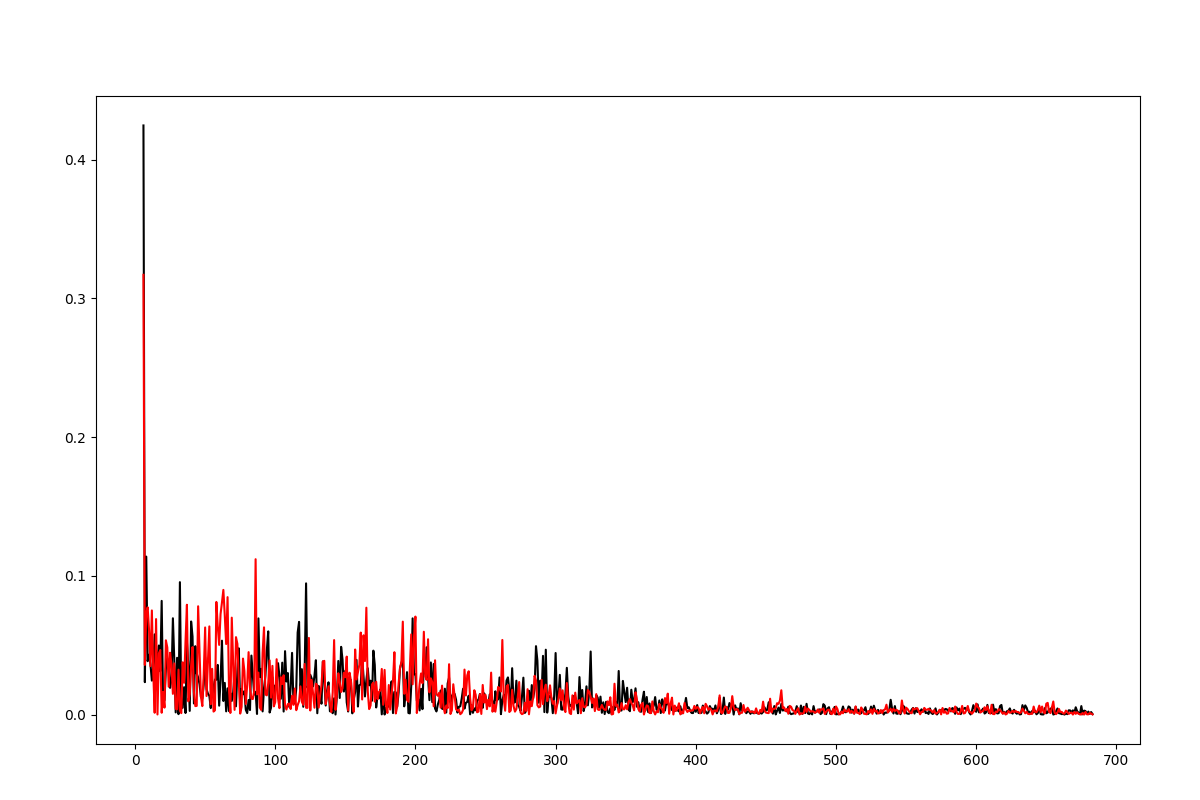
The distribution of the deformation in the distance contributed by each mode for a selected pair of residues has been described in [EB08], see Eq. (10) and plots are shown on Fig. (2).

These results can be plotted using plotting.showPairDeformationDist() or a list can be obtained using analysis.calcPairDeformationDist().

In [19]: d0 = calcPairDeformationDist(anm, calphas, 3, 132)

In [20]: show = showPairDeformationDist(anm, calphas, 3, 132)

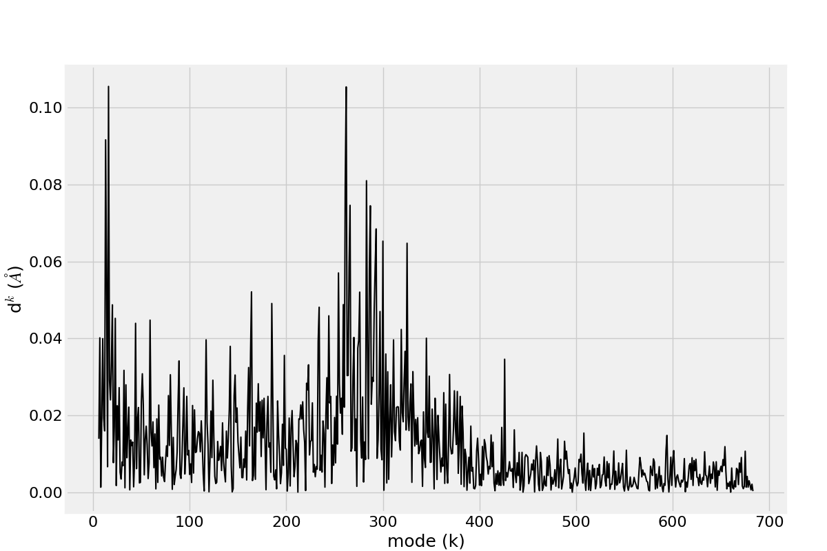
Figure shows the plotted distribution for deformations between 3-132 residue in each mode k.

To obtain results without saving any file type:

In [21]: d1 = calcPairDeformationDist(anm, calphas, 3, 212)

In [22]: d2 = calcPairDeformationDist(anm, calphas, 132, 212)

In [23]: plot(d1[0], d1[1], 'k-', d2[0], d2[1], 'r-')
Out[23]: 
[<matplotlib.lines.Line2D at 0x7f82c74fd050>,
 <matplotlib.lines.Line2D at 0x7f82c74fde90>]