Analysis
Here are the required imports again. You do not need to repeat them if you are still in the same python session.
In [1]: from prody import *

In [2]: from pylab import *

In [3]: ion()
You can load the model again if you are starting a new session as follows:
In [4]: anm_ampar = loadModel('3kg2.anm.npz')

In [5]: ampar_ca = parsePDB('3kg2', subset='ca')
Plotting effectiveness and sensitivity profiles
We can use showPerturbResponse with the matrix=False option to plot the effectiveness and sensitivity profiles colored by chain:
In [6]: show = showPerturbResponse(anm_ampar, atoms=ampar_ca,
   ...:                            show_matrix=False)
   ...:
Plotting residue-specific effectiveness and sensitivity profiles
To look at the effectiveness that perturbing a residue has in eliciting a response in individual residues (instead of its overall effectiveness) or to look at the sensitivity of a residue to perturbations of individual residues (instead of its overall sensitivity), we read out rows or columns from the perturbation response matrix. This can again be shown in a plot as in Figure 6D.
In [7]: show = showPerturbResponse(anm_ampar, atoms=ampar_ca,
   ...:                            show_matrix=False,
   ...:                            select='chain B and resnum 84')
   ...:
We can also calculate the PRS matrix and profiles separately from showPerturbResponse. This gives us more flexibility with what we show and enables us to do other things with the return values. For example, we could apply a cutoff to identify residues with particularly high effectiveness and sensitivity as effectors and sensors, or slice out individual rows or columns and write them into PDB files for visualization (see below).
In [8]: prs_mat, effectiveness, sensitivity = calcPerturbResponse(anm_ampar)
Writing effectiveness and sensitivity profiles to PDB for visualization
It is sometimes more helpful to understand what is happening using a colored structure. To achieve this we can overwrite the B-factor or occupancy column of PDB file and use PyMOL or VMD to color the structure by B-factor or occupancy.
To do this we modify the ampar_ca object and then write a PDB from it as follows:
In [9]: ampar_ca.setBetas(effectiveness)

In [10]: writePDB('3kg2_ca_effectiveness.pdb', ampar_ca)
Out[10]: '3kg2_ca_effectiveness.pdb'
We can also calculate the PRS matrix and profiles separately from showPerturbResponse and slice out individual rows or columns and write them into PDB files for visualization. We slice rows using axis=0 to obtain the effectiveness profile
In [11]: B_84_effectiveness = sliceAtomicData(prs_mat, atoms=ampar_ca, axis=0,
   ....:                                      select='chain B and resnum 84')
   ....:

In [12]: writePDB('3kg2_ca_B_84_effectiveness.pdb', ampar_ca,
   ....:          beta=B_84_effectiveness[0])
   ....:
Out[12]: '3kg2_ca_B_84_effectiveness.pdb'
and slice columns using axis=1 to obtain the sensitivity profile
In [13]: B_84_sensitivity = sliceAtomicData(prs_mat, atoms=ampar_ca, axis=1,
   ....:                                    select='chain B and resnum 84')
   ....:

In [14]: writePDB('3kg2_ca_B_84_sensitivity.pdb', ampar_ca,
   ....:          beta=B_84_sensitivity)
   ....:
Out[14]: '3kg2_ca_B_84_sensitivity.pdb'
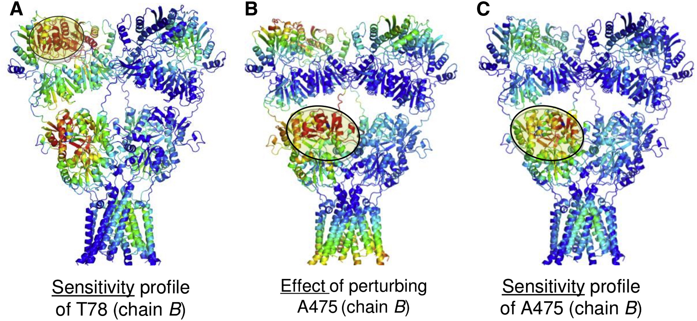
We generated our Figure 7 using this approach together with the spectrum command from PyMOL.