Overview

The first step in signature dynamics analysis is to collect a set of related protein structures and build a PDBEnsemble. This can be achieved by multiple routes: a query search of the PDB using blastPDB() or searchDali(), extraction of PDB IDs from the Pfam or CATH database, or input of a pre-defined list.

We demonstrate the Dali method here in the first part of the tutorial. The usage of Pfam and CATH methods are described in the database tutorial (under construction) and the function blastPDB() is described in the Structure Analysis Tutorial.

We apply these methods to the PBP-I domains, a group of protein structures originally found in bacteria for transport of solutes across the periplasmic space and later seen in various eukaryotic receptors including ionotropic and metabotropic glutamate receptors. We use the N-terminal domain of AMPA receptor subunit GluA2 (gene name GRIA2) as a query.

First, make necessary imports from ProDy and Matplotlib packages if you haven’t already.

In [1]: from prody import *

In [2]: from pylab import *

In [3]: ion()

Prepare ensemble (using Dali)

First we use the function searchDali() to search the PDB, which returns a DaliRecord object that contains a list of PDB IDs and their corresponding mappings to the reference structure.

In [4]: dali_rec = searchDali('3H5V','A')

In [5]: dali_rec
Out[5]: <prody.database.dali.DaliRecord at 0x7fb4fdb6fe50>

If DALI times out then, you can use the following code to fetch the data afterwards.

In [6]: while not dali_rec.isSuccess:
   ...:    dali_rec.fetch()
   ...: 

Next, we get the lists of PDB IDs and mappings from dali_rec, parse the pdb_ids to get a list of AtomGroup instances:

In [7]: pdb_ids = dali_rec.filter(cutoff_len=0.7, cutoff_rmsd=1.0, cutoff_Z=10)

In [8]: mappings = dali_rec.getMappings()

In [9]: ags = parsePDB(pdb_ids, subset='ca')

In [10]: len(ags)
Out[10]: 482

Then we provide ags together with mappings to buildPDBEnsemble(). We set the keyword argument seqid=20 to account for the low sequence identity between some of the structures.

In [11]: dali_ens = buildPDBEnsemble(ags, mapping=mappings, seqid=20)

In [12]: dali_ens
Out[12]: <PDBEnsemble: Unknown (69 conformations; 376 atoms)>

Finally we save the ensemble for later processing:

In [13]: saveEnsemble(dali_ens, 'PBP-I')
Out[13]: 'PBP-I.ens.npz'

Mode ensemble

For this analysis we’ll build a ModeEnsemble by calculating normal modes for each member of the PDBEnsemble. You can load a PDB ensemble at this stage if you already have one. We demonstrate this for the one we just saved.

In [14]: dali_ens = loadEnsemble('PBP-I.ens.npz')

Then we calculated GNM modes for each member of the ensemble. There are options to select the model (GNM by default) and the way of considering non-aligned residues by setting the trim option (default is reduceModel(), which treats them as environment).

In [15]: gnms = calcEnsembleENMs(dali_ens, model='GNM', trim='reduce')

In [16]: gnms
Out[16]: <ModeEnsemble: 69 modesets (20 modes, 376 atoms)>

We can also save the mode ensemble as follows:

In [17]: saveModeEnsemble(gnms, 'PBP-I')
Out[17]: 'PBP-I.modeens.npz'

We can load in a mode ensemble at this point as follows:

In [18]: gnms = loadModeEnsemble('PBP-I.modeens.npz')

Signature dynamics

Signatures are calculated as the mean and standard deviation of various properties such as mode shapes and mean square fluctations.

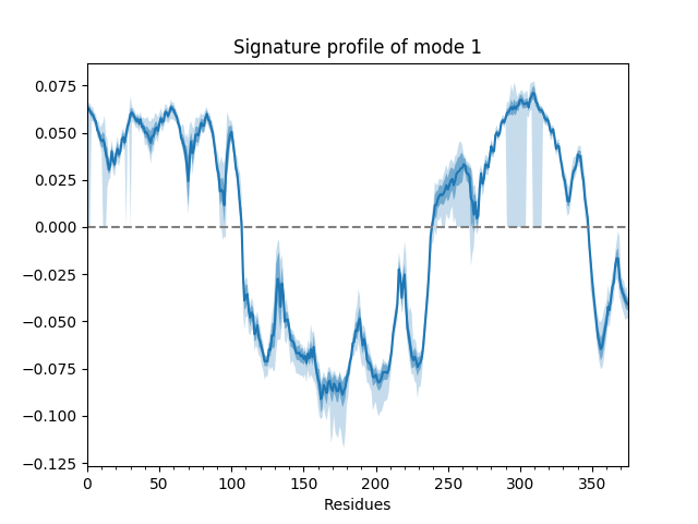
For example, we can show the average and standard deviation of the shape of the first mode (second index 0). The first index of the mode ensemble is over conformations.

In [19]: showSignatureMode(gnms[:, 0]);

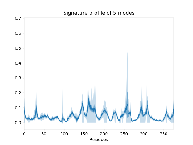
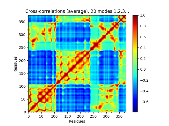
We can also show such results for properties involving multiple modes such as the mean square fluctuations from the first 5 modes or the cross-correlations from the first 20.

In [20]: showSignatureSqFlucts(gnms[:, :5]);

In [21]: showSignatureCrossCorr(gnms[:, :20]);

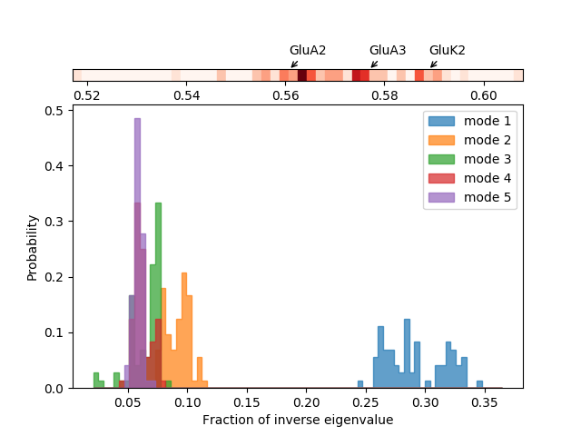
We can also look at distributions over values across different members of the ensemble such as inverse eigenvalue. We can show a bar above this with individual members labelled like [JK15].

We can select particular members to highlight with arrows by putting their names and labels in a dictionary:

In [22]: highlights = {'3h5vA_ca': 'GluA2','3o21C_ca': 'GluA3',
   ....:               '3h6gA_ca': 'GluK2', '3olzA_ca': 'GluK3',
   ....:               '5kc8A_ca': 'GluD2'}
   ....: 

We plot the variance bar for the first five modes (showing a function of the inverse eigenvalues related to the resultant relative size of motion) above the inverse eigenvalue distributions for each of those modes. To arrange the plots like this, we use the :class:~matplotlib.gridspec.GridSpec method of Matplotlib.

In [23]: from matplotlib.gridspec import GridSpec

In [24]: gs = GridSpec(ncols=1, nrows=2, height_ratios=[1, 10], hspace=0.15)

In [25]: subplot(gs[0]);

In [26]: showVarianceBar(gnms[:, :5], fraction=True, highlights=highlights);

In [27]: xlabel('');

In [28]: subplot(gs[1]);

In [29]: showSignatureVariances(gnms[:, :5], fraction=True, bins=80, alpha=0.7);

In [30]: xlabel('Fraction of inverse eigenvalue');

Spectral overlap and distance

Spectral overlap, also known as covariance overlap as defined in [BH02], measures the overlap between two covariance matrices, or the overlap of a subset of the modes (a mode spectrum).

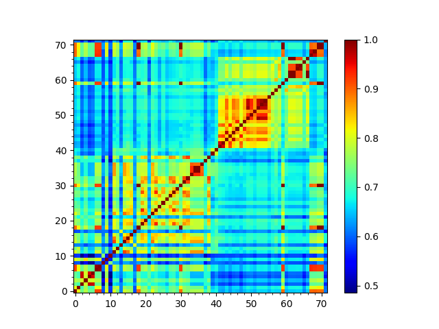
In [31]: so_matrix = calcEnsembleSpectralOverlaps(gnms[:, :1])

In [32]: showMatrix(so_matrix);

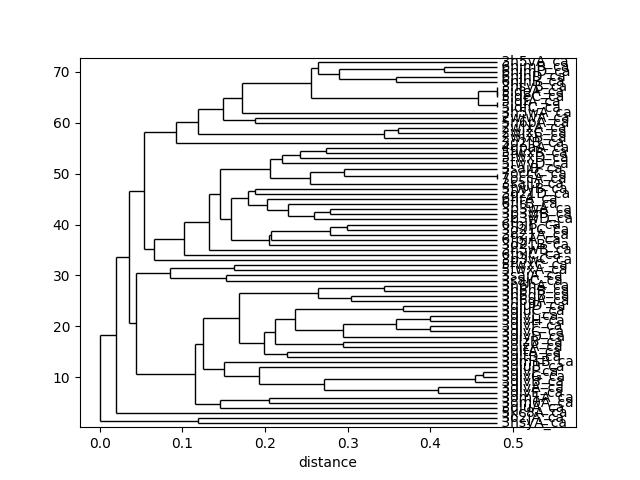
We can then calculate a tree from its arccosine, which converts the overlaps to distances:

In [33]: labels = gnms.getLabels()

In [34]: so_tree = calcTree(names=labels,
   ....:                    distance_matrix=arccos(so_matrix),
   ....:                    method='upgma')
   ....: 

This tree can be displaced using the :func:.showTree function. The default format is ASCII text but we can change it to plt to get a figure:

In [35]: showTree(so_tree, 'plt');

We can reorder the spectral overlap matrix using the tree as follows:

In [36]: reordered_so, new_so_indices = reorderMatrix(names=labels,
   ....:                                              matrix=so_matrix,
   ....:                                              tree=so_tree)
   ....: 

Both PDBEnsemble and ModeEnsemble objects can be reordered based on the new indices:

In [37]: reordered_ens = dali_ens[new_so_indices]

In [38]: reordered_gnms = gnms[new_so_indices, :]

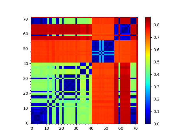
Comparing with sequence and structural distances

The sequence distance is given by the (normalized) Hamming distance, which is calculated by subtracting the percentage identity (fraction) from 1, and the structural distance is the RMSD. We can also calculate and show the matrices and trees for these from the PDB ensemble.

First we calculate the sequence distance matrix:

In [39]: seqid_matrix = buildSeqidMatrix(dali_ens.getMSA())

In [40]: seqdist_matrix = 1. - seqid_matrix

We can visualize the matrix using showMatrix():

In [41]: showMatrix(seqdist_matrix);

We can also construct a tree based on this distance matrix:

In [42]: seqdist_tree = calcTree(names=labels,
   ....:                         distance_matrix=seqdist_matrix,
   ....:                         method='upgma')
   ....: 

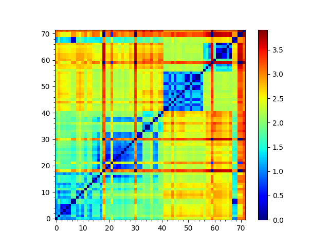
Similarily, once we obtain the RMSD matrix using PDBEnsemble.getRMSDs(), we can calculate the structure-based tree:

In [43]: rmsd_matrix = dali_ens.getRMSDs(pairwise=True)

In [44]: showMatrix(rmsd_matrix);

In [45]: rmsd_tree = calcTree(names=labels,
   ....:                      distance_matrix=rmsd_matrix,
   ....:                      method='upgma')
   ....: 

We could plot the three trees one by one. Or, it could be of interest to put all three trees constructed based on different distance metrics side by side and compare them:

In [46]: showTree(seqdist_tree, format='plt')

In [47]: title('Sequence')
Out[47]: Text(0.5,1,'Sequence')

In [48]: showTree(rmsd_tree, format='plt')

In [49]: title('Structure')
Out[49]: Text(0.5,1,'Structure')

In [50]: showTree(so_tree, format='plt')

In [51]: title('Dynamics')
Out[51]: Text(0.5,1,'Dynamics')

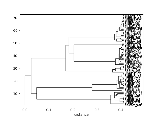
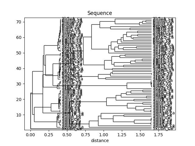
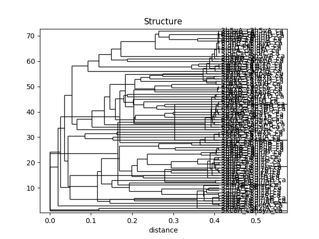
This analysis is quite sensitive to how many modes are used. As the number of modes approaches the full number, the dynamic distance order approaches the RMSD order. With smaller numbers, we see finer distinctions. This is particularly clear in the current case where we used just one mode.

[JK15]

Krieger J, Bahar I, Greger IH. Structure, Dynamics, and Allosteric Potential of Ionotropic Glutamate Receptor N-Terminal Domains. Biophys. J. 2015 109(6):1136-48