Simulation and Analysis
First, we will make the following necessary imports ProDy_, NumPy_, and Matplotlib_ if you haven’t already done it:
In [1]: import numpy as np

In [2]: import matplotlib.pyplot as plt

In [3]: from prody import *

In [4]: plt.ion()
Preparing the system and running a ClustENMD simulation
We start our calculations by parsing the structure, of which we would like to sample conformations. For this tutorial, we will fetch the X-Ray structure of HIV-1 protease in an open conformation in the absence of any inhibitor (PDB id: 1tw7) from the PDB server.
It is important to note that if the starting structure is provided by the user, it should satisfy the PDB file standards, e.g., the chain IDs need to be set properly.
The pdb file (PDB id: 1tw7) is fetched by the method parsePDB(). Please check the
ProDy Basics tutorials
for the details.
In [5]: pdb = parsePDB('1tw7', compressed=False)
@> PDB file is found in working directory (1tw7.pdb).
@> 1890 atoms and 1 coordinate set(s) were parsed in 0.03s.
ClustENMD is implemented as a ProDy class, named as ClustENM, so we can instantiate an object of it. You can provide a title, but it is optional.
In [6]: clustenm = ClustENM()
Before running a simulation, we need to set the atom group that we would like to use. This method uses PDBFixer to add all hydrogen atoms as well as any missing heavy atoms in any partially resolved residues. Note that even though PDBFixer can add any residues/segments that are not resolved in the PDB structure, we are not using this option of PDBFixer. Instead, we leave modeling of those parts to the user. User-provided models should include chain IDs in their PDB files.
At this step, you can also set the pH level of the solution to select the protonation states
for adding hydrogens by setting the pH parameter (default pH=7.0).
In [7]: clustenm.setAtoms(pdb)
@> Fixing the structure ...
@> 3108 atoms and 1 coordinate set(s) were parsed in 0.03s.
@> The structure was fixed in 1.91s.
After setting the atoms, you can write the fixed PDB file by the method ClustENM.writePDBFixed().
In [8]: clustenm.writePDBFixed()
A ClustENMD simulation is started by the ClustENM.run() method. This method accepts numerous
parameters, and we will only cover the essential ones to perform a simulation in this tutorial.
Therefore, we would like to encourage the readers to refer to the docstring of this method for
the description of all parameters.
As this method is iterative, the user needs to set the number of generations (default n_gens=5).
Depending on the system size, its flexibility, and the computational resources available, the user
can increase or decrease the number of generations. In this tutorial, we are using its default value.
The parameters regarding the main steps of the method can be grouped as follows:
ANM sampling:
cutoff: Cutoff distance for pairwise
interactions used in ANM computations (default is 15.0).
for pairwise
interactions used in ANM computations (default is 15.0).n_modes: Number of global modes for sampling (default is 3).n_confs: Number of new conformers generated from each parent conformer (default is 50).rmsds: RMSD of new conformers with
respect to the parent (default is 1.0).v1: Full enumeration of ANM modes, which is used in the original ClustENM method (default is False; see below).In the current ClustENMD version, ANM sampling is done randomly by the ProDy method
sampleModes, where the RMSD value corresponds to the average RMSD of the new conformers with respect to the parent conformer. As the bigger RMSD value yields larger excursions from the parent, the user should be cautious on increasing its value. In contrast the original ClustENM [KD16] uses the full enumeration (all possible combinations) of ANM modes with fixed maximum RMSD, which can be enabled by settingv1=True. In both cases, we suggest using the first 3 to 5 global modes as they are known to facilitate the conformational transitions.Clustering:
maxclust: Maximum number of clusters to be formed in each generation (default is None).threshold: RMSD threshold to apply when forming clusters (default is None).We are using SciPy hierarchical clustering library to cluster the conformers in each generation. Either
maxclustorthresholdparameter must be specified by the user. As a guideline, we suggest to use themaxclustparameter. Furthermore, the parameters can be not only set to a single value across the generations, but also provided exclusive to each generation as a tuple, e.g.,maxclust=(20, 40, 60). Increasing the number of maximum clusters in subsequent generations allows for maximum excursion from the initial structure, thus should be preferred.Relaxation via MD simulations:
temp: Temperature at which the simulation is conducted (default is 303.15 K).solvent: Solvent model to be used. Default is'imp', which corresponds to the implicit solvent model ('amber99sbildn.xml','amber99_obc.xml'). To choose the explicit solvent model ('amber14-all.xml','amber14/tip3pfb.xml'),solventshould be set to'exp'. The user may choose other force fields available in OpenMM, please see the description offorce_fieldparameter. However, only the default force-fields named above have been tested in ClustENMD so far. In the current implementation of ClustENMD, implicit solvent model is applicable to protein chains only. If there are any DNA/RNA chains in your structure, ClustENMD automatically uses explicit solvent.padding: Padding distance to be used for solvation (default is 1.0 nm).ionicStrength: Total concentration of ions (both positive and negative) to add. This does not include ions that are added to neutralize the system. Default concentration is 0.0 molar.tolerance: Energy tolerance to be used for performing a local energy minimization on the system (default is 10.0 kJ/mole).maxIterations: Maximum number of iterations to perform during energy minimization. If this is 0 (default), minimization is continued until the results converge without regard to how many iterations it takes.sim: A short MD simulation using a time step of 2.0 fs is performed ifsim=True. Note that there is also a heating-up phase until the desired temperature is reached before the short MD simulation. Ifsimis set to False, only energy minizimation is performed. If only a heating-up phase is to be performed, the parameterst_steps_iandt_steps_gshould be set to 0 withsim=True(please see below).t_steps_i: Number of simulation steps for the starting conformer, i.e. zeroth generation, (default is 1000).t_steps_g: Number of simulation steps for all conformers except the starting conformer, (default is 7500). If desired, time steps for subsequent generations can be varied and given as a tuple, e.g., (3000, 5000, 7000).platform: Achitecture on which the OpenMM runs (default is None). It can be chosen as'CUDA','OpenCL', or'CPU'. For efficiency,'CUDA'or'OpenCL'is highly recommended.
We suggest to use implicit solvation and GPU platform for computational efficiency. Default parameters are highly efficient on GPU platform for proteins comprising several thousand residues. For larger assemblies, the user may prefer: (i) to decrease the number of clusters and/or generations, (ii) to perform only energy minimization with/out heating-up phase, or (iii) to carefully shrink the padding distance in explicit solvent.
Performing a simulation
In the following, we will perform a ClustENMD simulation of 5 generations using the first 3 global modes. Relaxation of conformers is carried out in implicit solvent via energy minimization followed by a heating-up phase. We are conducting the simulation on a GPU platform. Simulation details will be printed out during execution.
In [9]: clustenm.run(n_modes=3, n_gens=5,
   ...:              maxclust=tuple(range(20, 120, 20)),
   ...:              sim=True, solvent='imp',
   ...:              t_steps_i=0, t_steps_g=0,
   ...:              platform='CUDA')
   ...:
@> Kirchhoff was built in 0.02s.
@> Generation 0 ...
@> Minimization & heating-up in generation 0 ...
@> Completed in 1.94s.
@> #-------------------/*\-------------------#
@> Generation 1 ...
@> Sampling conformers in generation 1 ...
@> Hessian was built in 0.07s.
@> 3 modes were calculated in 0.04s.
@> Parameter: rmsd = 1.00 A
@> Parameter: n_confs = 50
@> Modes are scaled by 24.611726681118544.
@> Clustering in generation 1 ...
@> Centroids were generated in 0.24s.
@> Minimization & heating-up in generation 1 ...
@> Structures were sampled in 33.37s.
@> #-------------------/*\-------------------#
@> Generation 2 ...
@> Sampling conformers in generation 2 ...
@> Hessian was built in 0.07s.
@> 3 modes were calculated in 0.08s.
@> Parameter: rmsd = 1.00 A
@> Parameter: n_confs = 50
@> Modes are scaled by 21.96801859205728.
@> Hessian was built in 0.06s.
@> 3 modes were calculated in 0.07s.
...
@> #-------------------/*\-------------------#
@> Generation 5 ...
@> Sampling conformers in generation 5 ...
@> Hessian was built in 0.06s.
@> 3 modes were calculated in 0.03s.
@> Parameter: rmsd = 1.00 A
@> Parameter: n_confs = 50
@> Modes are scaled by 19.25666801776903.
...
@> Clustering in generation 5 ...
@> Centroids were generated in 14.04s.
@> Minimization & heating-up in generation 5 ...
@> Structures were sampled in 174.84s.
@> #-------------------/*\-------------------#
@> Creating an ensemble of conformers ...
@> Ensemble was created in 0.00s.
@> All completed in 558.38s.
The generated conformers are stored in a ClustENM ensemble object. For future reference, the
parameters set for a simulation can be saved into a file by the method ClustENM.writeParameters():
In [10]: clustenm.writeParameters()
As ClustENM ensemble is actually a ProDy ensemble,
we can also save it by the saveEnsemble() method:
In [11]: saveEnsemble(clustenm)
'1tw7_clustenm.ens.npz'
We also provide a method, called ClustENM.writePDB(), to write the conformers into a PDB file. The
boolean parameter single (default is True) of this method controls whether the conformers
are stored as models in a single PDB file, or each of them are saved as a separate PDB file.
In [12]: clustenm.writePDB()
@> PDB file saved as 1tw7_clustenm.pdb
One can also load the previously saved ensemble by
In [13]: saved_clustenm = loadEnsemble('1tw7_clustenm.ens.npz')
Features of ClustENM ensembles
As we mentioned above, ClustENM class is derived from ProDy ensemble class, therefore the methods
defined for the latter, such as ClustENM.getCoordsets(), ClustENM.superpose() and
many more can apply to ClustENM objects as well. All conformers in generations ( )
are automatically superposed onto the initial/zeroth conformer based on C
)
are automatically superposed onto the initial/zeroth conformer based on C -atoms
during a ClustENMD simulation.
-atoms
during a ClustENMD simulation.
There are alternative ways of indexing the generated conformers. User can either index ClustENM
object by clustenm[3], which picks the 4th conformer (presumably the 2nd conformer in the
1st generation) or equivalently with the generation number and an index as clustenm[1, 2].
Note that indices start from 0.
Let’s check we obtain the same coordinates by two alternative methods:
In [14]: np.allclose(clustenm[3].getCoords(), clustenm[1, 2].getCoords())
True
A ClustENM object supports slicing as well. For example, if we want to select the 4th conformer for every generation, then we only need to specify the index of the conformer in the second slot and select all in the first slot. If the desired conformers are not available in a particular generation, then they will be skipped.
In [15]: clustenm[:, 3]
<ClustENM: 1tw7_clustenm (5 conformations; 3108 atoms)>
We can access the coordinates of these conformers by the ClustENM.getCoordsets() method:
In [16]: clustenm[:, 3].getCoordsets()
array([[[ -3.95957387,  32.35691799,  -4.37383242],
         [ -4.94566778,  32.35594469,  -4.59228821],
         [ -3.63788137,  31.46009385,  -4.70897438],
         ...,
         [ -2.37337274,  29.5071206 ,  -3.7201629 ],
         [ -1.39627789,  29.60381804,  -3.27034612],
         [ -7.98974581,  31.21050202,  -4.31887029]],

         [[ -6.89570222,  32.89490785,  -5.27764023],
         [ -7.80893237,  32.7297113 ,  -5.67617107],
         [ -6.31021832,  32.07285054,  -5.23854147],
         ...,
         [ -5.32171232,  30.53324814,  -3.46080742],
         [ -4.58778402,  30.86851485,  -2.74293152],
         [-10.41683474,  31.15561532,  -5.46381784]],

         [[ -6.3447726 ,  34.20123262,  -5.5673921 ],
         [ -7.22727328,  34.01664711,  -6.02260974],
         [ -5.82362403,  33.34645491,  -5.43376411],
         ...,
         [ -4.07602444,  31.36764316,  -4.08790043],
         [ -3.22430149,  31.72057964,  -3.52540378],
         [-10.13066977,  31.95881599,  -6.06925207]],

         [[ -6.03426394,  33.17008188,  -5.2525952 ],
         [ -6.90546384,  32.76869162,  -5.56882538],
         [ -5.41631979,  32.40739972,  -5.01477094],
         ...,
         [ -4.18322255,  30.96462084,  -3.54549089],
         [ -3.39843848,  31.42003303,  -2.95973127],
         [-10.00982495,  30.65422159,  -6.45285668]],

         [[ -5.90545369,  33.39176383,  -5.49324755],
         [ -6.79399411,  33.26907861,  -5.95751872],
         [ -5.56441284,  32.44150355,  -5.52143941],
         ...,
         [ -2.89975089,  29.95653924,  -5.45052765],
         [ -1.8757943 ,  30.2292032 ,  -5.24180161],
         [ -9.38759977,  30.58004821,  -5.53001208]]])
On the other hand, we may want to select all the conformers of a specific generation. It is then enough to set the index of the generation in the first slot and select all in the second slot.
In [17]: clustenm[3, :]
<ClustENM: 1tw7_clustenm (60 conformations; 3108 atoms)>
Analysing the results
We would like to show how the computed conformers populate the conformational space as regards the essential dynamics of the structure. For this aim, we perform a principal component analysis (PCA) on the generated ensemble. Next, we will project the conformers onto the space spanned by the first two PCs, which explain the highest variance of the ensemble. This can be done using ProDy ensemble analysis.
We are calculating PCs based on the C-atoms. This selection can be done directly
on the ClustENM object.
In [18]: clustenm.select('ca')
In [19]: clustenm
<ClustENM: 1tw7_clustenm (301 conformations; selected 198 of 3108 atoms)>
In [20]: pca_clustenm = PCA()

In [21]: pca_clustenm.buildCovariance(clustenm)

In [22]: pca_clustenm.calcModes()
@> Covariance is calculated using 301 coordinate sets.
@> Covariance matrix calculated in 0.016746s.
@> 20 modes were calculated in 0.06s.
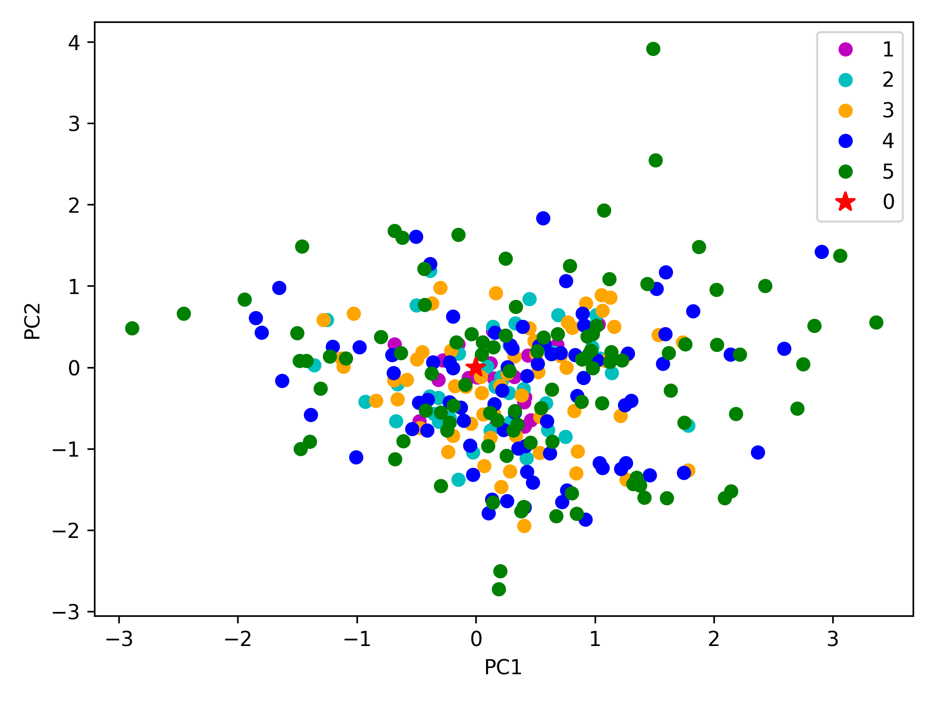
We can observe the progression of the conformers by coloring them in successive generations (from initial/zeroth to the last/fifth).
In [23]: with plt.style.context({'figure.dpi': 300,
   ....:                         'axes.labelsize': 'x-large',
   ....:                         'xtick.labelsize': 'large',
   ....:                         'ytick.labelsize': 'large'}):
   ....:     colors = ['r', 'm', 'c', 'orange', 'blue', 'green']
   ....:     plt.figure()
   ....:     for i in range(1, clustenm.numGenerations() + 1):
   ....:         showProjection(clustenm[i, :], pca_clustenm[:2],
   ....:                        c=colors[i], label='%d'%i)
   ....:     showProjection(clustenm[0, :], pca_clustenm[:2],
   ....:                    c=colors[0], label='0',
   ....:                    marker='*', markersize=10)
   ....:     plt.xlabel('PC1')
   ....:     plt.ylabel('PC2')
   ....:     plt.legend()
   ....:     plt.tight_layout()
   ....:     plt.show()
   ....:
The median and maximum RMSDs with respect to the initial conformer can be calculated for the whole ensemble by
In [24]: rmsds = clustenm.getRMSDs()
In [25]: np.median(rmsds), np.max(rmsds)
(1.6681441595969058, 4.407775779940453)
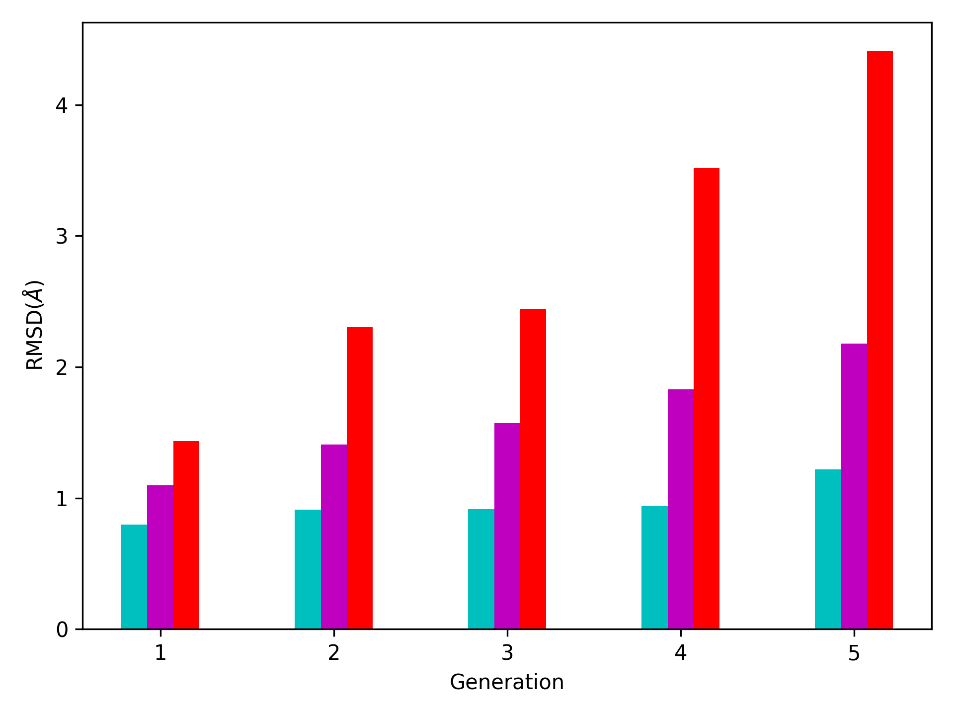
One can also check the RMSDs of the conformers in each generation with respect to the initial conformer:
In [26]: rmsd_gens = []

In [27]: for i in range(1, clustenm.numGenerations()+1):
   ....:     tmp = calcRMSD(clustenm.getCoords(),
   ....:                       clustenm[i, :].getCoordsets())
   ....:     rmsd_gens.append([tmp.min(), tmp.mean(), tmp.max()])
   ....:

In [28]: rmsd_gens = np.array(rmsd_gens)
In [29]: with plt.style.context({'figure.dpi': 300,
   ....:                         'axes.labelsize': 'x-large',
   ....:                         'xtick.labelsize': 'large',
   ....:                         'ytick.labelsize': 'large'}):
   ....:     plt.figure()
   ....:     plt.bar(np.arange(1, 6)-0.15, rmsd_gens[:, 0],
   ....:             width=.15, color='c', label='min')
   ....:     plt.bar(np.arange(1, 6), rmsd_gens[:, 1],
   ....:             width=.15, color='m', label='mean')
   ....:     plt.bar(np.arange(1, 6)+0.15, rmsd_gens[:, 2],
   ....:             width=.15, color='r', label='max')
   ....:     plt.xlabel('Generation')
   ....:     plt.ylabel(r'RMSD($\AA$)')
   ....:     plt.tight_layout()
   ....:     plt.show()
   ....:
We want to also observe if our conformers approach the closed state of HIV-1 protease. For this purpose, an NMR ensemble of 28 models (PDB ID: 1bve with closed flaps) is projected onto the same subspace.
Let’s first fetch these models and superpose them onto the initial/zeroth conformer. For this step, we generate a temporary ensemble of NMR models.
In [30]: closed = parsePDB('1bve', subset='ca', compressed=False)
@> PDB file is found in working directory (1bve.pdb).
@> 198 atoms and 28 coordinate set(s) were parsed in 0.10s.
In [31]: ens_cl = Ensemble()

In [32]: ens_cl.setAtoms(closed)

In [33]: ens_cl.setCoords(clustenm.getCoords())

In [34]: ens_cl.addCoordset(closed.getCoordsets())

In [35]: ens_cl.superpose()
@> Superposition completed in 0.03 seconds.
At this point, we will project both ClustENMD and NMR conformers on the subspace spanned by the first two PCs of the ClustENMD ensemble.
In [36]: with plt.style.context({'figure.dpi': 300,
   ....:                         'axes.labelsize': 'x-large',
   ....:                         'xtick.labelsize': 'large',
   ....:                         'ytick.labelsize': 'large'}):
   ....:     plt.figure()
   ....:     showProjection(clustenmd, pca_clustenmd[:2],
   ....:                       c='orange', markersize=5, alpha=.5, label='ClustENMD')
   ....:     showProjection(clustenmd[0], pca_clustenmd[:2],
   ....:                       c='r', marker='*', markersize=10, label='Initial')
   ....:     showProjection(ens_cl[2:], pca_clustenmd[:2],
   ....:                       markersize=5, c='c', label='1bve', alpha=.5)
   ....:     plt.xlabel('PC1')
   ....:     plt.ylabel('PC2')
   ....:     plt.legend()
   ....:     plt.tight_layout()
   ....:     plt.show()
   ....:
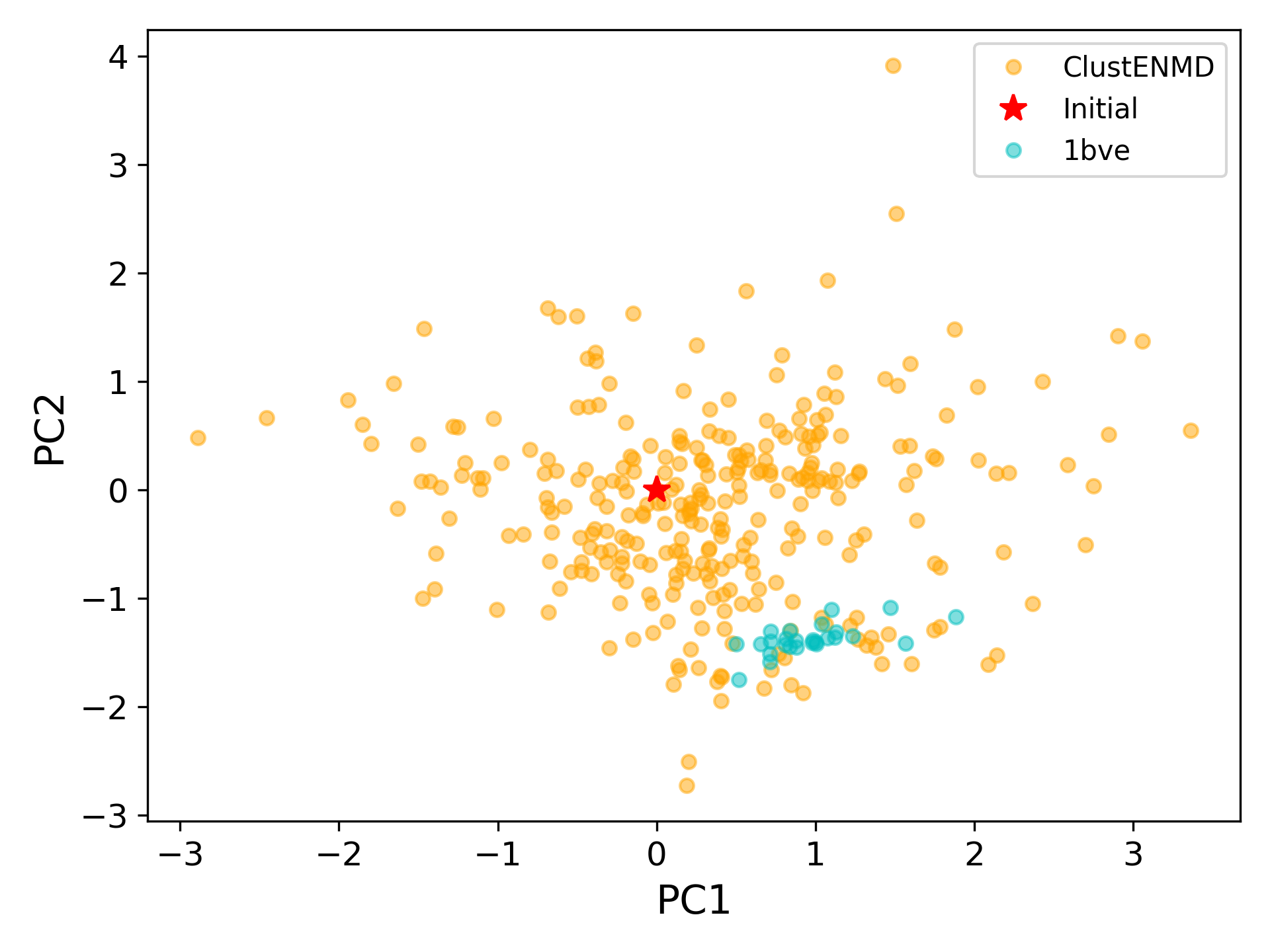
The figure above indicates that the unbiased conformer generation starting from the open state of HIV-1 protease (red star) can successfully encompass the NMR models representing its closed state (cyan dots). Each time you perform a ClustENMD run, you will obtain a unique ensemble due to the random sampling and MD simulations. Therefore, it is good practice to perform at least three independent runs, and combine the resulting ensembles for analysis.
Note: In this tutorial we showed the variability of our generated conformers following the procedure in our original paper [KD16]. An alternative approach could also be followed if there are enough experimentally resolved homologous structures representing alternative states of a flexible protein. In this approach, we can perform PCA on the ensemble of experimental structures and later project the ClustENMD conformers onto the subspace defined by PCs of experimental structures (see the examples in [KD21]). The movie on the ClustENMD webpage displays how the distribution, generated by a Gaussian kernel estimate plot, of HIV-1 protease conformational ensemble progresses as more generations are included. In that movie, ClustENMD conformers are projected on the experimental PC1 vs PC2. Specifically, blue surfaces/levels correspond to the progress of the runs starting from open structure.