Collective Molecular Dynamics Analysis

After running a coMD simulation, the results will be prepared in the same folder named in the setup section. You need to download the following files from that folder:

1. initial_ionized.pdb
2. final_ionized.pdb
3. initial_trajectory.dcd
4. final_trajectory.dcd

Preparing Trajectory Files

We recommend that you will follow this tutorial by typing commands in an IPython session, e.g.:

$ ipython

or with pylab environment:

$ ipython --pylab

First, we will make necessary imports from ProDy and Matplotlib packages.

In [1]: from prody import *

In [2]: from pylab import *

In [3]: ion()

coMD simulations will create two different trajectories and we need to use those two trajectories to analyze our simulations. However, the simulation boxes have different number of atoms due to the solvation and ionization procedure in the beginning of simulations. We therefore need to load trajectories with their related structure files.

In [4]: dcd1 = Trajectory('walker1_trajectory.dcd')

In [5]: dcd2 = Trajectory('walker2_trajectory.dcd')

In [6]: dcd1
Out[6]: <Trajectory: walker1_trajectory (next 0 of 40 frames; 29031 atoms)>

In [7]: dcd2
Out[7]: <Trajectory: walker2_trajectory (next 0 of 40 frames; 36588 atoms)>

In [8]: structure1 = parsePDB('walker1_ionized.pdb')

In [9]: structure2 = parsePDB('walker2_ionized.pdb')

In [10]: structure1
Out[10]: <AtomGroup: walker1_ionized (29031 atoms)>

In [11]: structure2
Out[11]: <AtomGroup: walker2_ionized (36588 atoms)>

In order to analyze the two trajectories together, we must have the same number of atoms in the sets that we analyze. To do this we link the trajectories to there corresponding initial structures and set the C-alpha atoms as the active ones with following commands:

In [12]: dcd1.setCoords(structure1)

In [13]: dcd1.setAtoms(structure1.calpha)

In [14]: dcd1
Out[14]: <Trajectory: walker1_trajectory (next 0 of 40 frames; selected 214 of 29031 atoms)>

In [15]: dcd2.setCoords(structure2)

In [16]: dcd2.setAtoms(structure2.calpha)

In [17]: dcd2
Out[17]: <Trajectory: walker2_trajectory (next 0 of 40 frames; selected 214 of 36588 atoms)>

Concatenating Trajectory Files

It is not possible to concatenate Trajectory objects inside Python but must instead be done using files. We therefore write out new files filtered to contain only C-alpha atoms as set in the previous step:

In [18]: writeDCD('initial_filtered.dcd', dcd1)
Out[18]: 'initial_filtered.dcd'

In [19]: writeDCD('final_filtered.dcd', dcd2)
Out[19]: 'final_filtered.dcd'

One way to combined trajectories into the same object is the addFile() method of Trajectory objects.

In [20]: traj = Trajectory('initial_filtered.dcd')

In [21]: traj.addFile('final_filtered.dcd')

Alternatively we can create an Ensemble using parseDCD(), which gives us the flexibility to do things like reversing the final trajectory to create something we can view in VMD rather than having the trajectories both run towards the shared intermediate. We do this as follows:

In [22]: combined_traj = parseDCD('initial_filtered.dcd')

In [23]: w2_traj = parseDCD('final_filtered.dcd')

In [24]: for i in reversed(range(len(w2_traj))):
   ....:     combined_traj.addCoordset(w2_traj.getConformation(i))
   ....: 

In [25]: combined_traj.superpose()

In [26]: writeDCD('combined_trajectory.dcd', combined_traj)
Out[26]: 'combined_trajectory.dcd'

We also write out a pdb file containing just the C-alpha atoms, which can be loaded into VMD together with this combined trajectory for visualization.

In [27]: writePDB('initial_filtered.pdb', structure1.ca)
Out[27]: 'initial_filtered.pdb'

Principal Component Analysis

We next perform PCA on the concatenated trajectory as follows.

In [28]: pca = PCA('Adelynate Kinase coMD')

In [29]: pca.buildCovariance(combined_traj)

In [30]: pca.calcModes()

The first half of the trajectory is from the initial structure and the second half of the trajectory is from the final structure. We can identify these two trajectories as follows.

In [31]: forward = combined_traj[0:40]

In [32]: backward = combined_traj[40:]

Visualization of Trajectories

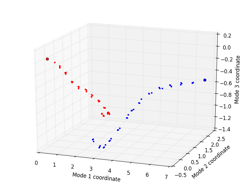
Finally, the trajectories can be plotted by using the showProjection() function:

In [33]: showProjection(forward, pca[:3], color='red', marker='.');

In [34]: showProjection(backward, pca[:3], color='blue', marker='.');

In [35]: showProjection(forward[0], pca[:3], color='red', marker='o');

In [36]: showProjection(backward[0], pca[:3], color='blue', marker='o');

The plots will be in the following form:

Having calculated the modes, we can write them to a .nmd file for viewing in NMWiz.

In [37]: writeNMD('ake_pca.nmd', pca, structure1.ca)
Out[37]: 'ake_pca.nmd'