ANM Calculations

Required imports:

In [1]: from prody import *

In [2]: from pylab import *

In [3]: ion()

Atom Selection

First, we parse p38 structure p38.pdb:

In [4]: p38 = parsePDB('conformational_sampling_files/p38.pdb')

In [5]: p38
Out[5]: <AtomGroup: p38 (5658 atoms)>

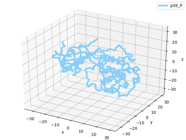
Let’s take a look at the structure:

In [6]: showProtein(p38);

In [7]: legend();

Note that this structure has hydrogen atoms which were added using PSFGEN that comes with NAMD:

In [8]: p38.numAtoms('hydrogen')
Out[8]: 2824

We will perform ANM calculations for 351 Cα atoms of the structure:

In [9]: p38_ca = p38.ca

In [10]: p38_ca
Out[10]: <Selection: 'ca' from p38 (351 atoms)>

ANM Calculation

First, let’s instantiate an ANM object:

In [11]: p38_anm = ANM('p38 ca')

In [12]: p38_anm
Out[12]: <ANM: p38 ca (0 modes; 0 nodes)>

Now, we can build Hessian matrix, simply by calling ANM.buildHessian() method:

In [13]: p38_anm.buildHessian(p38_ca)

In [14]: p38_anm
Out[14]: <ANM: p38 ca (0 modes; 351 nodes)>

We see that ANM object contains 351 nodes, which correspond to the Cα atoms.

We will calculate only top ranking three ANM modes, since we are going to use only that many in sampling:

In [15]: p38_anm.calcModes(n_modes=3)

In [16]: p38_anm
Out[16]: <ANM: p38 ca (3 modes; 351 nodes)>

Analysis & Plotting

Let’s plot mobility of residues along ANM modes:

In [17]: showSqFlucts(p38_anm);

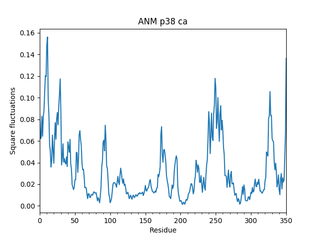
We can also calculate collectivity of these modes as follows:

In [18]: for mode in p38_anm:
   ....:     print('{}\tcollectivity: {}'.format(str(mode), calcCollectivity(mode)))
   ....: 
Mode 1 from ANM p38 ca	collectivity: 0.618084923455
Mode 2 from ANM p38 ca	collectivity: 0.585153336557
Mode 3 from ANM p38 ca	collectivity: 0.634434845453

Visualization

You can visualize ANM modes using Normal Mode Wizard. You need to write an .nmd file using writeNMD() and open it using VMD:

In [19]: writeNMD('p38_anm.nmd', p38_anm, p38_ca)
Out[19]: 'p38_anm.nmd'

For visualization, you can use viewNMDinVMD(), i.e. viewNMDinVMD('p38_anm.nmd')

Extend Model

We want to use the ANM model to sample all atoms conformations of p38 MAPK, but we have a coarse-grained model. We will use extendModel() function for this purpose:

In [20]: p38_anm_ext, p38_all = extendModel(p38_anm, p38_ca, p38, norm=True)

In [21]: p38_anm_ext
Out[21]: <NMA: Extended ANM p38 ca (3 modes; 5658 atoms)>

In [22]: p38_all
Out[22]: <AtomMap: AtomGroup p38 from p38 (5658 atoms)>

Note p38_anm_ext is an NMA model, which has similar features to an ANM object. This extended model still has 3 modes, but 5668 atoms as opposed to 351 nodes in the original ANM model.

Let’s plot mobility of residues again to help understand what extending a model does:

In [23]: showSqFlucts(p38_anm_ext);

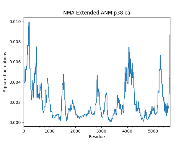
As you see, the shape of the mobility plot is identical. In the extended model, each atom moves in the same direction as the Cα atoms of the residue to which they belong. The mobility profile is scaled down, however, due to renormalization of the mode vectors.

Save Results

Now let’s save the original and extended model, and atoms:

In [24]: saveAtoms(p38)
Out[24]: 'p38.ag.npz'

In [25]: saveModel(p38_anm)
Out[25]: 'p38_ca.anm.npz'

In [26]: saveModel(p38_anm_ext, 'p38_ext')
Out[26]: 'p38_ext.nma.npz'

More Examples

We have performed a quick ANM calculation and extended the resulting model to all atoms of of the structure. You can see more examples on this in Elastic Network Models tutorial.