Processing Cryo-EM Electron Density Maps

Let’s start with essential import statements:

In [1]: from prody import *

In [2]: import numpy as np

Parse Density Map

The first step is to parse a .map file, which contains information about a density map as the electron density at points on a grid. This file format is a binary format also known as CCP4 or MRC2014.

We provide parameters to return pseudoatom beads from the electron density map using the Topology Representing Network algorithm.

Note: Depending on your hardware and the system size, this may take a while. To skip this step, you can load the structure file for the beads directly in PDB format (EMD-1961.pdb; see below).

In [3]: emd = parseEMD('1961', cutoff=1.2, n_nodes=3000)

In [4]: emd

This function returns an AtomGroup from the electron density map. The cutoff parameter discards any electron density lower than the given number and we select this based on the suggestion on the `EMDB`_ website. In this case, we raise it slightly to remove unassigned density inside the CCT rings.

The parameter n_nodes describes the total number of beads in the system, which we choose to be a few times smaller than the number of residues to increase efficiency and account for the low resolution.

This procedure is an iterative one and num_iter can be used to set the number of them (the default value is 20).

The resultant structure will look something like the following figure.

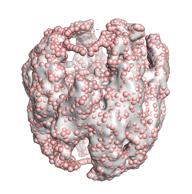
Now that the 144x144x144 density grid is converted into an AtomGroup object, elastic network model analysis can be applied to the constructed structure as usual.

Map pseudo-atoms to PDB atomic model

To save time, you may parse pseudo-atoms from a PDB file generated as above. We also parse the PDB model for comparison later.

In [5]: emd = parsePDB('EMD-1961.pdb')

In [6]: pdb = parsePDB('4a0v', subset='ca')

The order of pseudo-atoms generated by TRN is random and does not follow a sequence like residues in an atomic model do. Also, they have no chain identifiers. For the purpose of visualization and later comparative analyses, we reorder the pseudo-atoms and assign the residue and chain identifers to the pseudo-atoms based on the PDB structure in the following section.

Unique one-to-one mapping of pseudo-atoms to an atomic model is nontrivial, since there is no correspondence between the beads and the residues of the protein. For simplicity, here we use the k-nearest neighbors algorithm to find 20 closest residues in the atomic model to a given pseudo-atom. Then we create a one-to-one mapping by assigning the closest residue, or the next closest if it is already assigned, to a pseudo-atom. Note that this is by no means the optimal one-to-one mapping, and for more complicated methods which guarantees the optimal mapping, see for example the “stable marriage problem”.

In [7]: from sklearn.neighbors import NearestNeighbors

In [8]: mapping = []

In [9]: nbrs = NearestNeighbors(n_neighbors=20, algorithm='ball_tree').fit(pdb.getCoords())

In [10]: _, indices = nbrs.kneighbors(emd.getCoords())

In [11]: for neighbors in indices:
   ....:    for i in neighbors:
   ....:       if i not in mapping:
   ....:          mapping.append(i)
   ....:          break
   ....: 

In [12]: indices = np.array(mapping)

In [13]: I = np.argsort(indices)

Note that indices returned from NearestNeighbors is a 2-D array with rows corresponding to pseudo-atoms and columns their k-neighbors. After being processed by the for-loop above, each element of indices is the index of the residue in the atomic model that should be assigned to the pseudo-atom. Then, argsort() is applied to obtain indices for reordering the pseudo-atoms following the order of the atoms (residues) in the atomic model.

We first create a AtomMap for the atomic model with only the residues that were mapped to a pseudo-atom.

In [14]: pmap = AtomMap(pdb, indices[I])

Then we create a new AtomGroup for the pseudo-atoms based on the mapping, such that they are ordered according to the sequence of residues they are assigned to:

In [15]: emd2 = AtomMap(emd, I).toAtomGroup()

In [16]: resnums = pmap.getResnums()

In [17]: emd2.setResnums(resnums)

In [18]: chids = pmap.getChids()

In [19]: emd2.setChids(chids)

Now we can calculate the RMSD between the pseudo-atoms and their mapped residues in the atomic model:

In [20]: calcRMSD(emd2, pmap)
Out[20]: 3.30205562866952

Finally, we save the ordered pseudo-atom model to a PDB file for visualization and other downstream analyses:

In [21]: writePDB('EMD-1961_mapped.pdb', emd2)
Out[21]: 'EMD-1961_mapped.pdb'

Elastic Network Model Analysis

Elastic network model analysis can be applied to the pseudo-atomic model as usual. We use cutoff=20 to account for the level of coarse-graining (see [PD02]).

[PD02]

P. Doruker, R.L. Jernigan, I. Bahar, Dynamics of large proteins through hierarchical levels of coarse-grained structures, J. Comput. Chem. 2002 23:119-127.

In [22]: anm_emd = ANM('TRiC EMDMAP ANM Analysis')

In [23]: anm_emd.buildHessian(emd2, cutoff=20)

In [24]: anm_emd.calcModes(n_modes=5)

In [25]: writeNMD('tric_anm_3_modes_3000nodes.nmd', anm_emd[:3], emd2)
Out[25]: 'tric_anm_3_modes_3000nodes.nmd'

Compare results with atomic models

For comparison, let’s perform ENM analysis for the atomic model (i.e. pmap we created earlier) as well, and apply the reduced model to it to treat residues that are not assigned to a pseudo-atom as the environment.

In [26]: anm_pdb = ANM('4a0v ANM')

In [27]: anm_pdb.buildHessian(pdb)

In [28]: anm_pdb_reduced, _ = reduceModel(anm_pdb, pdb, pmap)

In [29]: anm_pdb_reduced.calcModes(n_modes=5)

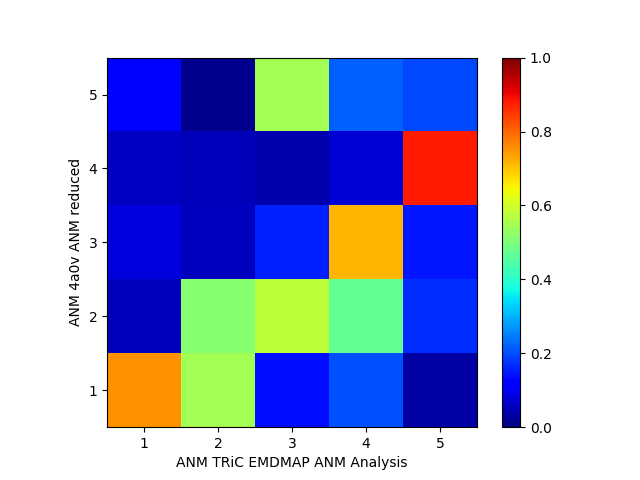
Now we compare modes of the pseudo-atomic model to the atomic model:

In [30]: showOverlapTable(anm_emd, anm_pdb_reduced)
Out[30]: 
(<matplotlib.image.AxesImage at 0x7f844187c050>,
 [],
 <matplotlib.colorbar.Colorbar at 0x7f843fe7f790>)