Editing a Model

This example shows how to analyze the normal modes corresponding to a system of interest. In this example, ANM calculations will be performed for HIV-1 reverse transcriptase (RT) subunits p66 and p51. Analysis will be made for subunit p66. Output is a reduced/sliced model that can be used as input to analysis and plotting functions.

ANM calculations

We start by importing everything from the ProDy package:

In [1]: from prody import *

In [2]: from matplotlib.pylab import *

In [3]: ion()

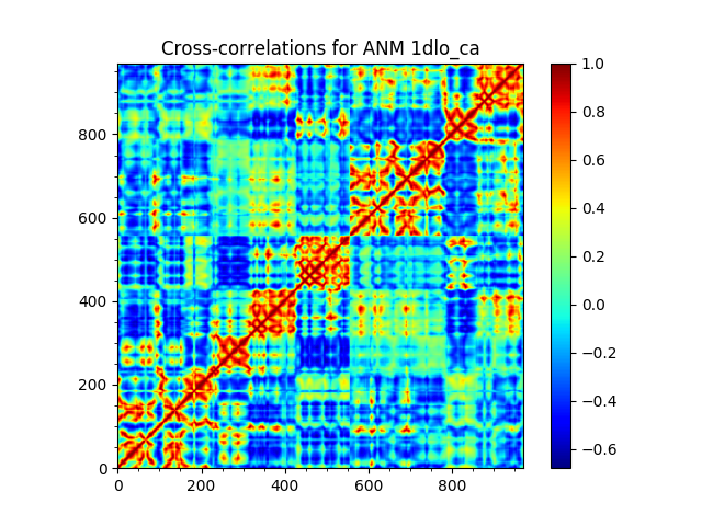
We start with parsing the Cα atoms of the RT structure 1DLO and performing ANM calculations for them:

In [4]: rt = parsePDB('1dlo', subset="ca")

In [5]: anm, sel = calcANM(rt)

In [6]: anm
Out[6]: <ANM: 1dlo_ca (20 modes; 971 nodes)>

In [7]: saveModel(anm, 'rt_anm')
Out[7]: 'rt_anm.anm.npz'

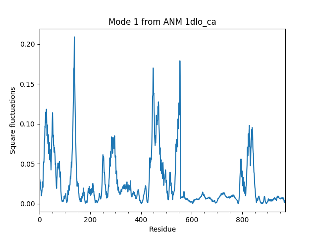
In [8]: anm[:5].getEigvals().round(3)
Out[8]: array([0.039, 0.063, 0.126, 0.181, 0.221])

In [9]: (anm[0].getArray() ** 2).sum() ** 0.5
Out[9]: 0.9999999999999999

Analysis

We can plot the cross-correlations and square fluctuations for the full model as follows:

Cross-correlations

In [10]: showCrossCorr(anm);

Square fluctuations

In [11]: showSqFlucts(anm[0]);

Slicing a model

Slicing a model is analogous to slicing a list, i.e.:

In [12]: numbers = list(range(10))

In [13]: numbers
Out[13]: [0, 1, 2, 3, 4, 5, 6, 7, 8, 9]

In [14]: slice_first_half = numbers[:10]

In [15]: slice_first_half
Out[15]: [0, 1, 2, 3, 4, 5, 6, 7, 8, 9]

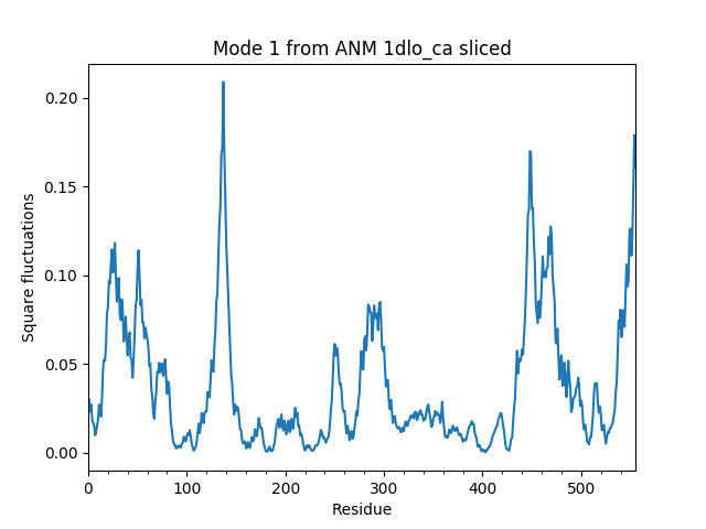
In this case, we want to slice normal modes, so that we will handle mode data corresponding to subunit p66, which is chain A in the structure. We use sliceModel() function:

In [16]: anm_slc_p66, sel_p66 = sliceModel(anm, rt, 'chain A')

In [17]: anm_slc_p66
Out[17]: <ANM: 1dlo_ca sliced (20 modes; 556 nodes)>

You see that now the sliced model contains 556 nodes out of the 971 nodes in the original model.

In [18]: saveModel(anm_slc_p66, 'rt_anm_sliced')
Out[18]: 'rt_anm_sliced.anm.npz'

In [19]: anm_slc_p66[:5].getEigvals().round(3)
Out[19]: array([0.039, 0.063, 0.126, 0.181, 0.221])

In [20]: '%.3f' % (anm_slc_p66[0].getArray() ** 2).sum() ** 0.5
Out[20]: '0.895'

Note that slicing does not change anything in the model apart from taking parts of the modes matching the selection. The sliced model contains fewer nodes, has the same eigenvalues, and modes in the model are not normalized.

Analysis

We plot the cross-correlations and square fluctuations for the sliced model in the same way. Note that the plots contain the selected part of the model without any change:

Cross-correlations

In [21]: showCrossCorr(anm_slc_p66);

In [22]: title('Cross-correlations for ANM slice');

Square fluctuations

In [23]: showSqFlucts(anm_slc_p66[0]);

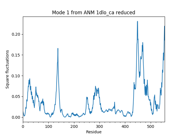
Reducing a model

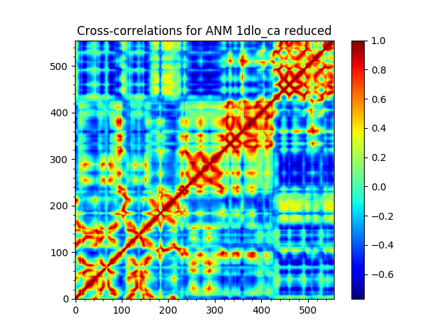
We reduce the ANM model to subunit p66 using reduceModel() function. This function implements the method described in 2000 paper of Hinsen et al. [KH00]

In [24]: anm_red_p66, sel_p66 = reduceModel(anm, rt, 'chain A')

In [25]: anm_red_p66.calcModes()

In [26]: anm_red_p66
Out[26]: <ANM: 1dlo_ca reduced (20 modes; 556 nodes)>

In [27]: saveModel(anm_red_p66, 'rt_anm_reduced')
Out[27]: 'rt_anm_reduced.anm.npz'

In [28]: anm_red_p66[:5].getEigvals().round(3)
Out[28]: array([0.05 , 0.098, 0.214, 0.289, 0.423])

In [29]: '%.3f' % (anm_red_p66[0].getArray() ** 2).sum() ** 0.5
Out[29]: '1.000'

Analysis

We plot the cross-correlations and square fluctuations for the reduced model in the same way. Note that in this case the plots are not identical to the full model:

Cross-correlations

In [30]: showCrossCorr(anm_red_p66);

Square fluctuations

In [31]: showSqFlucts(anm_red_p66[0]);

Compare reduced and sliced models

We can compare the sliced and reduced models by plotting the overlap table between modes:

In [32]: showOverlapTable(anm_slc_p66, anm_red_p66);

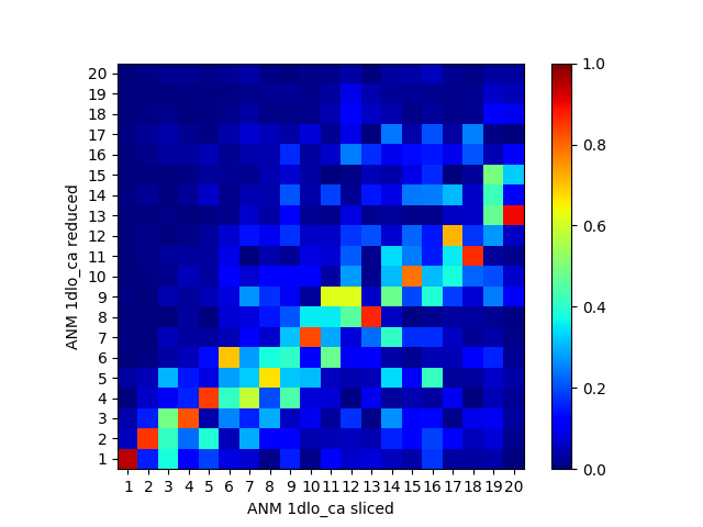
The sliced and reduced models are not the same. While the purpose of slicing is simply enabling easy plotting/analysis of properties of a part of the system, reducing has other uses as in [WZ05].

[WZ05]

Zheng W, Brooks BR. Probing the Local Dynamics of Nucleotide-Binding Pocket Coupled to the Global Dynamics: Myosin versus Kinesin. Biophysical Journal 2005 89:167–178.