Calculations and Analysis
First, we will make necessary imports from ProDy, NumPy, Matplotlib, and Pandas packages if you haven’t already done it:
In [1]: from prody import *

In [2]: from numpy import *

In [3]: from matplotlib.pyplot import *

In [4]: from pandas import *

In [5]: ion()
Generation of ESSA profile
First, we parse a structure on which we want to perform ESSA. For this tutorial, we will fetch the TEM-1 beta-lactamase (1pzo) from the PDB.
In [6]: ag = parsePDB('1pzo', compressed=False)
ESSA is implemented as a ProDy class, so we can instantiate an ESSA
object.
In [7]: essa = ESSA()
Before starting residue scanning, we first need to set the system. Even though
the ligand(s) are not included in the scanning, they can be specified for further
analysis. For this purpose, users can simply give the chain ids and residue numbers
as a string shown in the following. The protein residues interacting with each ligand
can be determined within a specific cutoff distance (default dist=4.5).
ESSA will use the title of the atomic object provided to it in the names of the
output files.
ESSA, by default, generates a ModeEnsemble containing the modes
resulting from the perturbation of each residue. However, if the user does not
have enough memory resources for conducting computation on a large structure,
then lowmem=True should be chosen, thus only storing eigenvalues/eigenvectors
for each perturbed model.
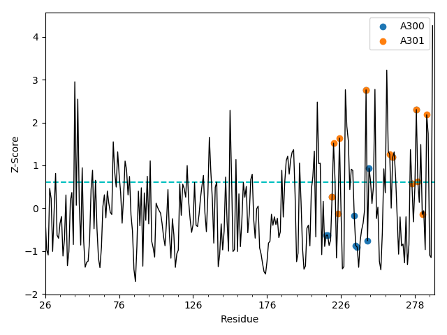
In the structure 1pzo, there are two identical allosteric inhibitors (residues 300 and 301 of chain A). ESSA can be informed about them when setting the system as follows:
In [8]: essa.setSystem(ag, lig='A 300 A 301')
Scanning can be done using scanResidue(). Here one can specify the number
of softest modes, the type of ENM (GNM or ANM), and the cutoff, which by default
are n_modes=10, enm='gnm', cutoff=None, respectively. If cutoff
is not specified, its value is adopted from the default value of the specified ENM.
During the scanning, the progress will also be displayed.
In [9]: essa.scanResidues()
The generated ESSA profile can be shown by showESSAProfile(). On this profile,
the residues interacting with the previously specified ligand(s) are automatically
highlighted. The blue dashed baseline shows the q-th quantile of the profile, which is by
default q=0.75, representing the top quartile. Other residues of interest
can also be indicated with their single-letter code and residue number on this plot
if specified by a ProDy selection string provided as a parameter. Users can dynamically
customize the properties of the plot using the matplotlib context manager as shown below.
In [10]: with style.context({'figure.dpi': 100}):
   ....:     essa.showESSAProfile()
   ....:

ESSA z-scores can be obtained as a NumPy array using getESSAZscores(), and saved with
saveESSAZscores(). Let’s have the z-scores of the first ten residues:
In [11]: essa.getESSAZscores()[:10]
Out[11]:
array([-0.24676638, -0.97356457, -1.09135811,  0.46199512,  0.22145561,
       -1.00814207, -0.06428016,  0.812289  , -0.62965247, -0.70051851])
In [12]: essa.saveESSAZscores()
In order to visualize the essential residues, a PDB file can be generated, in which the z-scores are written in the B-factor column. Later, this file can be opened in a molecular graphics program such as PyMOL or VMD, where the structure can be colored according to the B-factors.
In [13]: essa.writeESSAZscoresToPDB()
Please check the other getter and save methods and their docstrings, such as those for ligand binding residues.
Prediction of allosteric pockets
Allosteric pocket prediction requires Fpocket 3.0 and Pandas installed in your
system. The first step is the pocket hunting, which is automatically carried out
in the background, by calling scanPockets(). This method parses the pocket
features provided by Fpocket, and all identified pockets are stored in a folder
ending with _out in the current working directory. Additionally, maximum/median
ESSA scores are assigned to each pocket based on the ESSA scores of the residues
forming it.
In [14]: essa.scanPockets()
Pocket features that are stored in a Pandas DataFrame can be obtained by
getPocketFeatures(), and saved as a Python pickle file by
savePocketZscores().
Key features of the pockets to be used in the prediction, namely ESSA and local
hydrophobic density (LHD) z-scores, can be listed by getPocketZscores().
In [15]: essa.getPocketZscores()
Out[15]:
Z-score   ESSA_max  ESSA_med       LHD
Pocket #
1         1.051557 -0.748037 -0.674785
2         0.571688 -0.293197 -0.314441
3         1.137016 -0.332065 -0.068207
4         2.283472  0.283524 -0.134270
5         1.137016  0.579200 -0.674785
6         2.773325  0.392536  2.386841
7         0.177499 -1.011726 -0.520354
The prediction protocol ranks the pockets with respect to their ESSA and LHD z-scores. Concurrently, the pockets with negative LHD z-scores are filtered out as allosteric sites are known to have relatively higher LHD. For the details of this protocol, please refer to the original ESSA article [KB20].
Ranking of the pockets can be performed and obtained by rankPockets() and
getPocketRanks(), respectively.
In [16]: essa.rankPockets()

In [17]: essa.getPocketRanks()
Out[17]:
      Pocket # (ESSA_max & LHD)  Pocket # (ESSA_med & LHD)
Rank
1                             6                          6
Pocket 6 with the top ESSA_max score has been identified as the only allosteric pocket in this structure. Interestingly, other pockets have been filtered out due to their negative LHD z-scores. Pocket 6 is a large pocket that includes CBT allosteric ligands at A300 and A301, as well as a part of the orthosteric ligand (see Figure S2 and Table S2 of [KB20]).
In order to visualize the pockets, the .pqr file, an output of Fpocket needs to be opened by PyMOL or VMD together with the original pdb file.
Pocket z-scores and ranks can be saved by savePocketZscores() and
writePocketRanksToCSV(), respectively.
In [18]: essa.savePocketZscores()

In [19]: essa.writePocketRanksToCSV()
