Classification using sequence, structure and dynamics distances
We can compare the dynamics of individual proteins using the spectral overlap, also known as covariance overlap. The arccosine of this value provides a distance metric. Calculating this for all pairs in a mode ensemble gives us the spectral distance matrix, which can be used to calculate a dynamics-based “phylogenetic” tree. This can be compared against matrices and trees calculated using sequence and structure distances.
Again here are the imports if you need them.
In [1]: from prody import *

In [2]: from pylab import *

In [3]: ion()
Load PDBEnsemble and ModeEnsemble
We first load the PDBEnsemble:
In [4]: ens = loadEnsemble('LeuT.ens.npz')
Then we load the ModeEnsemble:
In [5]: gnms = loadModeEnsemble('LeuT.modeens.npz')
Spectral overlap and distance
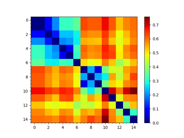
We calculate a distance matrix based on spectral overlaps (calculated as their arccosines), calculate a tree from it and reorder the matrix using the tree as follows:
In [6]: sd_matrix = calcEnsembleSpectralOverlaps(gnms[:,:1], distance=True)

In [7]: labels = gnms.getLabels()

In [8]: so_tree = calcTree(names=labels,
   ...:                   distance_matrix=sd_matrix,
   ...:                   method='upgma')
   ...:

In [9]: reordered_sd, new_sd_indices = reorderMatrix(names=labels,
   ...:                                              matrix=sd_matrix,
   ...:                                              tree=so_tree)
   ...:
We can show the original and reordered spectral distance matrices and the tree as follows.
showTree() has multiple format options. Here we show the output of using plt.
This layout allows us to directly compare against the output from showMatrix()
using the option origin=’upper’.
In [10]: showMatrix(sd_matrix, origin='upper');

In [11]: showTree(so_tree, format='plt');

In [12]: showMatrix(reordered_sd, origin='upper');


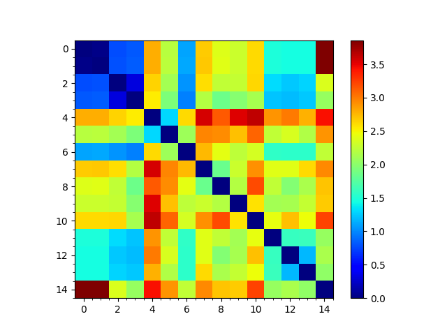
Sequence and structural distances
The sequence distance is given by the Hamming distance, which is calculated by subtracting the percentage identity (fraction) from 1, and the structural distance is the RMSD. We can also calculate and show the matrices and trees for these from the PDB ensemble.
In [13]: seqid_matrix = buildSeqidMatrix(ens.getMSA())

In [14]: seqd_matrix = 1. - seqid_matrix

In [15]: showMatrix(seqd_matrix, origin='upper');

In [16]: seqd_tree = calcTree(names=labels,
   ....:                      distance_matrix=seqd_matrix,
   ....:                      method='upgma')
   ....:

In [17]: showTree(seqd_tree, format='plt');

In [18]: reordered_seqd, indices = reorderMatrix(labels, seqd_matrix, seqd_tree)

In [19]: showMatrix(reordered_seqd, origin='upper');


In [20]: rmsd_matrix = ens.getRMSDs(pairwise=True)

In [21]: showMatrix(rmsd_matrix, origin='upper');

In [22]: rmsd_tree = calcTree(names=labels,
   ....:                      distance_matrix=rmsd_matrix,
   ....:                      method='upgma')
   ....:

In [23]: showTree(rmsd_tree, format='plt');

In [24]: reordered_rmsd, indices = reorderMatrix(labels, rmsd_matrix, rmsd_tree)

In [25]: showMatrix(reordered_rmsd, origin='upper');


Comparing sequence, structural and dynamic classifications
We can reorder the seqd and sod matrices by the RMSD tree too to compare them:
In [26]: reordered_seqd, indices = reorderMatrix(names=labels, matrix=seqd_matrix, tree=rmsd_tree)

In [27]: reordered_sd, indices = reorderMatrix(names=labels, matrix=sd_matrix, tree=rmsd_tree)
In [28]: showMatrix(reordered_seqd, origin='upper')
Out[28]:
(<matplotlib.image.AxesImage at 0x7fb50268d990>,
 [],
 <matplotlib.colorbar.Colorbar at 0x7fb500234790>)

In [29]: showMatrix(reordered_rmsd, origin='upper')
Out[29]:
(<matplotlib.image.AxesImage at 0x7fb50258d7d0>,
 [],
 <matplotlib.colorbar.Colorbar at 0x7fb4fedfb710>)

In [30]: showMatrix(reordered_sd, origin='upper')
Out[30]:
(<matplotlib.image.AxesImage at 0x7fb4fed48990>,
 [],
 <matplotlib.colorbar.Colorbar at 0x7fb4fed1c910>)


This analysis is quite sensitive to how many modes are used. As the number of modes approaches the full number, the dynamic distance order approaches the RMSD order. With smaller numbers, we see finer distinctions. This is particularly clear in the current case where we used just one mode.