Sequence-Structure Comparison
The part shows how to compare sequence conservation properties with structural mobility obtained from Gaussian network model (GNM) calculations.
In [1]: from prody import *

In [2]: from matplotlib.pylab import *

In [3]: ion()  # turn interactive mode on
Entropy Calculation
First, we retrieve MSA for protein for protein family PF00074:
In [4]: fetchPfamMSA('PF00074')
Out[4]: 'PF00074_full.sth'
We parse the MSA file:
In [5]: msa = parseMSA('PF00074_full.sth')
Then, we refine it using refineMSA() based on the sequence of
RNAS1_BOVIN:
In [6]: msa_refine = refineMSA(msa, label='RNAS1_BOVIN', seqid=0.98)
We calculate the entropy for the refined MSA:
In [7]: entropy = calcShannonEntropy(msa_refine)
Mobility Calculation
Next, we obtain residue fluctuations or mobility for protein member of the above family. We will use chain B of 2W5I.
In [8]: pdb = parsePDB('2W5I', chain='B')
We can use the function alignSequenceToMSA() to identify the part of
the PDB file that matches with the MSA. In cases where this fails, a label
keyword argument can be provided to the function as well.
In [9]: aln, idx_1, idx_2 = alignSequenceToMSA(pdb, msa_refine, label='RNAS1_BOVIN')

In [10]: showAlignment(aln, indices=[idx_1, idx_2])

               	                  20        30        40        50        60
2W5IB          	KETAAAKFERQHMDSSTSAASSSNYCNQMMKSRNLTKDRCKPVNTFVHESLADVQAVCSQ

               	                  18        28        38        48        58
RNAS1_BOVIN    	--TAAAKFERQHMDSSTSAASSSNYCNQMMKSRNLTKDRCKPVNTFVHESLADVQAVCSQ


               	        70        80        90       100       110       120
2W5IB          	KNVACKNGQTNCYQSYSTMSITDCRETGSSKYPNCAYKTTQANKHIIVACEGNPYVPVHF

               	        68        78        88        98       108       118
RNAS1_BOVIN    	KNVACKNGQTNCYQSYSTMSITDCRETGSSKYPNCAYKTTQANKHIIVACEGNPYVPVHF


2W5IB          	DASV


RNAS1_BOVIN    	D---
This tells us that the first two residues are missing as are the last three, ending the sequence at residue 121. Hence, we make a selection accordingly:
In [11]: chB = pdb.select('resnum 3 to 121')
We can see from the sequence that this gives us the right portion:
In [12]: chB.ca.getSequence()
Out[12]: 'TAAAKFERQHMDSSTSAASSSNYCNQMMKSRNLTKDRCKPVNTFVHESLADVQAVCSQKNVACKNGQTNCYQSYSTMSITDCRETGSSKYPNCAYKTTQANKHIIVACEGNPYVPVHFD'
We write this selection to a PDB file for use later, e.g. with evol apps.
In [13]: writePDB('2W5IB_3-121.pdb', chB)
Out[13]: '2W5IB_3-121.pdb'
We perform GNM as follows:
In [14]: gnm = GNM('2W5I')

In [15]: gnm.buildKirchhoff(chB.ca)

In [16]: gnm.calcModes(n_modes=None)  # calculate all modes
Now, let’s obtain residue mobility using the slowest mode, the slowest 8 modes, and all modes:
In [17]: mobility_1 = calcSqFlucts(gnm[0])

In [18]: mobility_1to8 = calcSqFlucts(gnm[:8])

In [19]: mobility_all = calcSqFlucts(gnm[:])
See Gaussian Network Model (GNM) for details.
Comparison of mobility and conservation
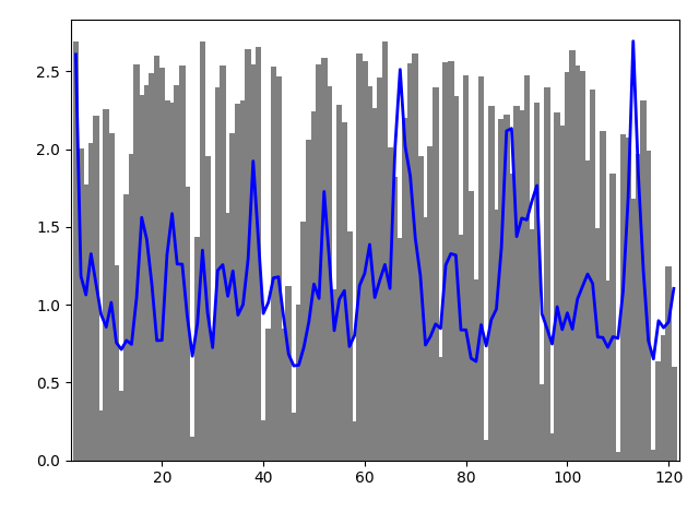
We use the above data to compare structural mobility and degree of conservation. We can calculate a correlation coefficient between the two quantities:
In [20]: result = corrcoef(mobility_all, entropy)

In [21]: result.round(3)[0,1]
Out[21]: 0.396
We can plot the two curves simultaneously to visualize the correlation. We have to scale the values of mobility to display them in the same plot.
Plotting
In [22]: indices = chB.ca.getResnums()

In [23]: bar(indices, entropy, width=1.2, color='grey');

In [24]: xlim(min(indices)-1, max(indices)+1);

In [25]: plot(indices, mobility_all*(max(entropy)/max(mobility_all)), color='b',
   ....: linewidth=2);
   ....:
Writing PDB files
We can also write PDB with b-factor column replaced by entropy and mobility values respectively. We can then load the PDB structure in VMD or PyMol to see the distribution of entropy and mobility on the structure.
In [26]: selprot = chB.copy()

In [27]: resindex = selprot.getResindices()

In [28]: entropy_prot = [entropy[ind] for ind in resindex]

In [29]: mobility_prot = [mobility_all[ind]*10 for ind in resindex]

In [30]: selprot.setBetas(entropy_prot)

In [31]: writePDB('2W5I_entropy.pdb', selprot)
Out[31]: '2W5I_entropy.pdb'

In [32]: selprot.setBetas(mobility_prot)

In [33]: writePDB('2W5I_mobility.pdb', selprot)
Out[33]: '2W5I_mobility.pdb'
We can see on the structure just as we could in the bar graph that there is some correlation with highly conserved (low entropy) regions having low mobility and high entropy regions have higher mobility.