Implicit Membrane ANM
Here we will make use of ProDy’s implicit membrane ANM (imANM) capabilities to investigate the motions of a
neurotransmitter transporter in the presence of the plasma membrane. The procedure is based on the methods
described in [TL12] and relies on the Rotations and Translations of Blocks (RTB) method [FT00]
of reducing complexity within ENMs. To follow this tutorial, you will need the following files:
- Membrane-aligned outward-facing structure file (2NWL-opm.pdb)
- Membrane-aligned inward-facing structure file (3KBC-opm.pdb)
- Outward-facing block definition file (2nwl_blocks.txt)
- Inward-facing block definition file (3kbc_blocks.txt)
These files can be downloaded from one of the following links:
The first file contains the outward-facing structure of the glutamate transporter after insertion into the plasma membrane. It is obtained from the Orientations of Proteins in Membranes database.
| [TL12] | Lezon TR, Bahar I. Constraints Imposed by the Membrane Selectively Guide the Alternating Access Dynamics of the Glutamate Transporter GltPh. Biophys J 2012 102 1331-1340. |
| [FT00] | Tama F, Gadea FJ, Marques O, Sanejouand YH. Building-block approach for determining low-frequency normal modes of macromolecules. Proteins 2000 41 1-7. |
Preparing the structures
Begin by firing up ProDy in the usual manner:
In [1]: from prody import *

In [2]: from pylab import *

In [3]: ion()
The imANM assumes that the membrane is normal to the z-axis, so it is important to use a structure that is properly aligned. The structure from the OPM database will work.
In [4]: of_all = parsePDB('2NWL-opm.pdb')  # Outward-facing structure

In [5]: if_all = parsePDB('3KBC-opm.pdb')  # Inward-facing structure
There will be warnings saying that ProDy wants to read beta factors, but the coordinates should be read properly. In addition to atoms, the OPM file contains points to indicate the boundaries of the membrane.
We now make two selections, one from each structure. The selections are chosen so that the final structures are homotrimers with an equal number (398) of atoms in each subunit. We also want to remove the three aspartate ligands, which are indicated as chain D in the outward-facing structure and have resid 500, in the inward-facing structure.
In [6]: of_ca = of_all.select('protein and name CA and not ((chain A and resid 119 to 122) or (chain C and resid 119 to 123) or chain D)')

In [7]: if_ca = if_all.select('protein and name CA and not (resid 6 to 9 119 to 127) and resid < 500')
As a last step in preparation, we can align the structures so that we can calculate a deformation vector and compare the modes to it, as shown in the ENM Tutorial.
In [8]: superpose(if_ca, of_ca)
Out[8]:
(<Selection: 'protein and nam...and resid < 500' from 3KBC-opm (1194 atoms)>,
 <prody.measure.transform.Transformation at 0x7f82c7a19520>)
Assigning Blocks
imANM is an extension of ProDy’s RTB method, which can be used for any system, whether or not a membrane is involved. The RTB method allows us to decompose the protein into pre-defined rigid blocks. Atoms within a block do not move relative to each other (hence the descriptor “rigid”), but blocks can move relative to other blocks. There are two main benefits of using blocks: First, the Hessian for a good blocking scheme is smaller than the Hessian for an all-residue representation, so the modes can be calculated more quickly. This is particularly useful when one is considering very large systems (in this case, containing thousands of residues). Second, the use of rigid blocks reduces unphysical distortions of the structure, such as stretching of backbone bonds that may result from the harmonic approximation. These benefits come at the price of accuracy. Imposing rigidity reduces the amount of dynamical detail that can be recovered from the model.
In ProDy, a rigid block is defined as a set of atoms that move together (i.e., the distances between them are fixed). Typically the constituent atoms of a rigid block are spatially adjacent (i.e., they all belong to the same domain or secondary structure element), but users are free to define blocks however they wish. The only restriction is that a block cannot contain exactly two particles. This restriction is in place because it is mathematically inconvenient to deal with two-particle blocks.
We can either define blocks within our python session, or define them externally in a separate file and write a little bit of code to handle the tasks of
reading the file and assigning residues to blocks. This latter approach can be useful when exploring and comparing many different blocking schemes.
We have developed one such format for a block file, examples of which can be found in 2nwl_blocks.txt and 3kbc_blocks.txt.
The first ten lines of 2nwl_blocks.txt are:
1 TYR A     10  VAL A     12
4 LEU A     13  LYS A     15
5 ILE A     16  TYR A     33
6 GLY A     34  ALA A     36
7 HIS A     37  VAL A     43
8 LYS A     44  ALA A     70
9 ALA A     71  ALA A     71
10 SER A     72  SER A     72
11 ILE A     73  ILE A     73
12 SER A     74  LEU A     78
The columns, separated by whitespace, are formatted as follows:
- Integer identifier of the block.
- Three-letter code for first residue in the block.
- Chain ID of first residue in the block.
- Resnum of first residue in the block.
- Three-letter code for last residue in the block.
- Chain ID of last residue in block.
- Resnum of last residue in the block.
This is just one way of storing information on how the protein is deconstructed into blocks. You are welcome to use others if you have a way of reading them.
We can read blocks from 2nwl_blocks.txt into of_ca and the array of_blocks as follows:
In [9]: blk='2nwl_blocks.txt'

In [10]: ag = of_ca.getAtomGroup()

In [11]: ag.setData('block', 0)

In [12]: with open(blk) as inp:
   ....:    for line in inp:
   ....:       b, n1, c1, r1, n2, c2, r2 = line.split()
   ....:       sel = of_ca.select('chain {} and resnum {} to {}'
   ....:                          .format(c1, r1, r2))
   ....:       if sel != None:
   ....:          sel.setData('block', b)
   ....:

In [13]: of_blocks = of_ca.getData('block')
We will do the same for the blocks of the inward-facing structure. The block definitions are based on secondary structures, which vary slightly between the structures. We therefore have two separate blocking schemes.
In [14]: blk = '3kbc_blocks.txt'

In [15]: ag = if_ca.getAtomGroup()

In [16]: ag.setData('block', 0)

In [17]: with open(blk) as inp:
   ....:    for line in inp:
   ....:       b, n1, c1, r1, n2, c2, r2 = line.split()
   ....:       sel = if_ca.select('chain {} and resnum {} to {}'
   ....:                          .format(c1, r1, r2))
   ....:       if sel != None:
   ....:          sel.setData('block', b)
   ....:

In [18]: if_blocks = if_ca.getData('block')
Calculating the Modes
To use the blocks in an RTB imANM calculation, we instantiate an imANM object for each structure:
In [19]: of_imanm = imANM('2nwl')

In [20]: if_imanm = imANM('3kbc')
and we build a couple of Hessians using the coordinates of the crystal structures.
In [21]: of_coords = of_ca.getCoords()

In [22]: if_coords = if_ca.getCoords()

In [23]: of_imanm.buildHessian(of_coords, of_blocks, scale=16., depth=27.)

In [24]: if_imanm.buildHessian(if_coords, if_blocks, scale=16., depth=27.)
The scaling factor of 16 in this example means that the restoring force for any displacement in the x- or y-direction is 16 times greater than the force associated with a displacement in the z-direction. The constraint on motions parallel to the membrane surface implicitly incorporates the membrane’s effects into ANM.
The parameter depth specifies the total size of the membrane in the
z direction, half of which goes either side of the x-y plane. It is also
possible to set the positions of the upper and lower edges of the membrane
separately using high and low.
Next we calculate the modes and write them to a pair of .nmd files for viewing.
In [25]: of_imanm.calcModes()

In [26]: if_imanm.calcModes()

In [27]: writeNMD('2nwl_im.nmd', of_imanm, of_ca.select('protein and name CA'))
Out[27]: '2nwl_im.nmd'

In [28]: writeNMD('3kbc_im.nmd', if_imanm, if_ca.select('protein and name CA'))
Out[28]: '3kbc_im.nmd'
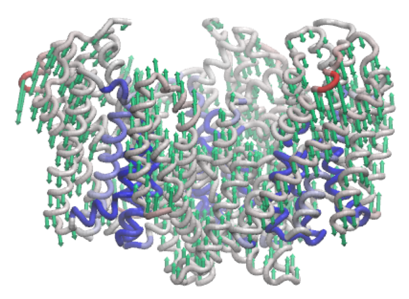
The third mode of the outward-facing structure moves all three transport domains simultaneously through the membrane in a ‘lift-like’ motion.
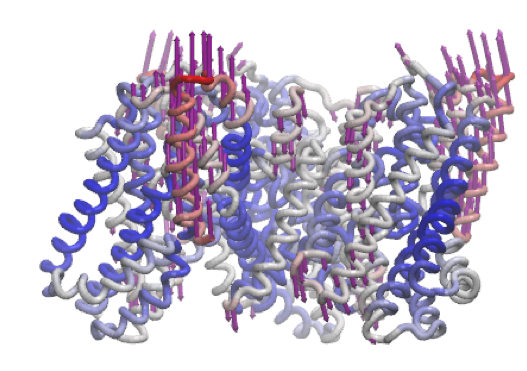
A similar motion is shown in mode 6 of the inward-facing structure.