Dynamics Analysis
In this section, we will show how to perform quick PCA and ANM analysis using a solution structure of Ubiquitin. If you started a new Python session, import ProDy contents:
In [1]: from prody import *

In [2]: from pylab import *

In [3]: ion()
PCA Calculations
Let’s perform principal component analysis (PCA) of an ensemble
of NMR models, such as 2k39. The same example is presented in the
Ensemble Analysis where more details are provided.
First, we prepare the ensemble:
In [4]: ubi = parsePDB('2k39', subset='calpha')

In [5]: ubi_selection = ubi.select('resnum < 71')

In [6]: ubi_ensemble = Ensemble(ubi_selection)

In [7]: ubi_ensemble.iterpose()
Then, we perform the PCA calculations:
In [8]: pca = PCA('Ubiquitin')

In [9]: pca.buildCovariance(ubi_ensemble)

In [10]: pca.calcModes()
This analysis provides us with a description of the dominant changes in the structural ensemble. Let’s see the fraction of variance for top ranking 4 PCs:
In [11]: for mode in pca[:4]:
   ....:     print(calcFractVariance(mode).round(2))
   ....:
0.13
0.09
0.08
0.07
PCA data can be saved on disk using saveModel() function:
In [12]: saveModel(pca)
Out[12]: 'Ubiquitin.pca.npz'
This function writes data in binary format, so is an efficient way of
storing data permanently. In a later session, this data can be loaded using
loadModel() function.
ANM Calculations
Anisotropic network model (ANM) analysis can be
performed in two ways:
The shorter way, which may be suitable for interactive sessions:
In [13]: anm, atoms = calcANM(ubi_selection, selstr='calpha')
The longer and more controlled way:
In [14]: anm = ANM('ubi') # instantiate ANM object

In [15]: anm.buildHessian(ubi_selection) # build Hessian matrix for selected atoms

In [16]: anm.calcModes() # calculate normal modes

In [17]: saveModel(anm)
Out[17]: 'ubi.anm.npz'
Anisotropic Network Model (ANM) provides a more detailed discussion of ANM calculations.
The above longer way gives more control to the user. For example, instead of
building the Hessian matrix using uniform force constant and cutoff distance,
customized force constant functions (see Custom Gamma Functions) or a pre-calculated
matrix (see ANM.setHessian()) may be used.
Individual Mode instances can be accessed by
indexing the ANM instance:
In [18]: slowest_mode = anm[0]

In [19]: print( slowest_mode )
Mode 1 from ANM ubi

In [20]: print( slowest_mode.getEigval().round(3) )
1.714
Note that indices in Python start from zero (0). 0th mode is the 1st non-zero mode in this case. Let’s confirm that normal modes are orthogonal to each other:
In [21]: (anm[0] * anm[1]).round(10)
Out[21]: -0.0

In [22]: (anm[0] * anm[2]).round(10)
Out[22]: -0.0
As you might have noticed, multiplication of two modes is nothing but the
dot() product of mode vectors/arrays. See
Normal Mode Algebra for more examples.
Comparative Analysis
ProDy comes with many built-in functions to facilitate a comparative analysis
of experimental and theoretical data. For example, using
printOverlapTable() function you can see the agreement between
experimental (PCA) modes and theoretical (ANM) modes calculated above:
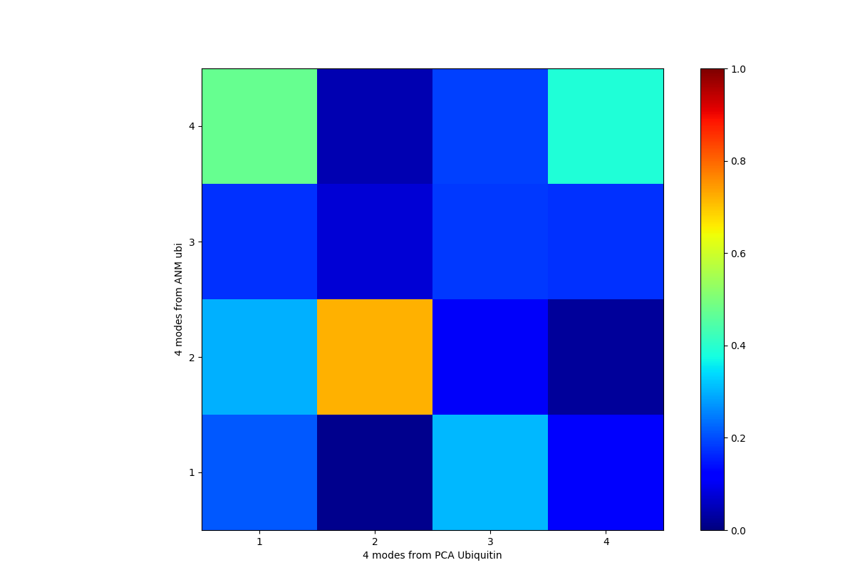
In [23]: printOverlapTable(pca[:4], anm[:4])
Overlap Table
                            ANM ubi
                     #1     #2     #3     #4
PCA Ubiquitin #1   -0.21  +0.30  -0.17  -0.47
PCA Ubiquitin #2   +0.01  +0.72  +0.08  +0.05
PCA Ubiquitin #3   +0.31  +0.11  +0.18  +0.19
PCA Ubiquitin #4   +0.11  -0.02  -0.17  -0.39
Output above shows that PCA mode 2 and ANM mode 2 for ubiquitin show the highest overlap (cosine-correlation).
In [24]: showOverlapTable(pca[:4], anm[:4]);
This was a short example for a simple case. Ensemble Analysis section contains more comprehensive examples for heterogeneous datasets. Analysis shows more analysis function usage examples and Dynamics Analysis module documentation lists all of the analysis functions.
Output Data Files
The writeNMD() function writes PCA results in NMD format.
NMD files can be viewed using the Normal Mode Wizard VMD plugin.
In [25]: writeNMD('ubi_pca.nmd', pca[:3], ubi_selection)
Out[25]: 'ubi_pca.nmd'
Additionally, results can be written in plain text files for analysis with
other programs using the writeArray() function:
In [26]: writeArray('ubi_pca_modes.txt', pca.getArray(), format='%8.3f')
Out[26]: 'ubi_pca_modes.txt'
External Data
Normal mode data from other NMA, EDA, or PCA programs can be parsed using
parseModes() function for analysis.
In this case, we will parse ANM modes for p38 MAP Kinase calculated using
ANM server as the external software.
We use oanm_eigvals.txt and oanm_slwevs.txt files from
the ANM server.
You can either download these files to your current working directory from here or obtain them for another protein from the ANM server.
In [27]: nma = parseModes(normalmodes='oanm_slwevs.txt',
....: eigenvalues='oanm_eigvals.txt',
....: nm_usecols=range(1,21), ev_usecols=[1], ev_usevalues=range(6,26))
....:
In [28]: nma
Out[28]: <NMA: oanm_slwevs (20 modes; 351 atoms)>
In [29]: nma.setTitle('1p38 ANM')
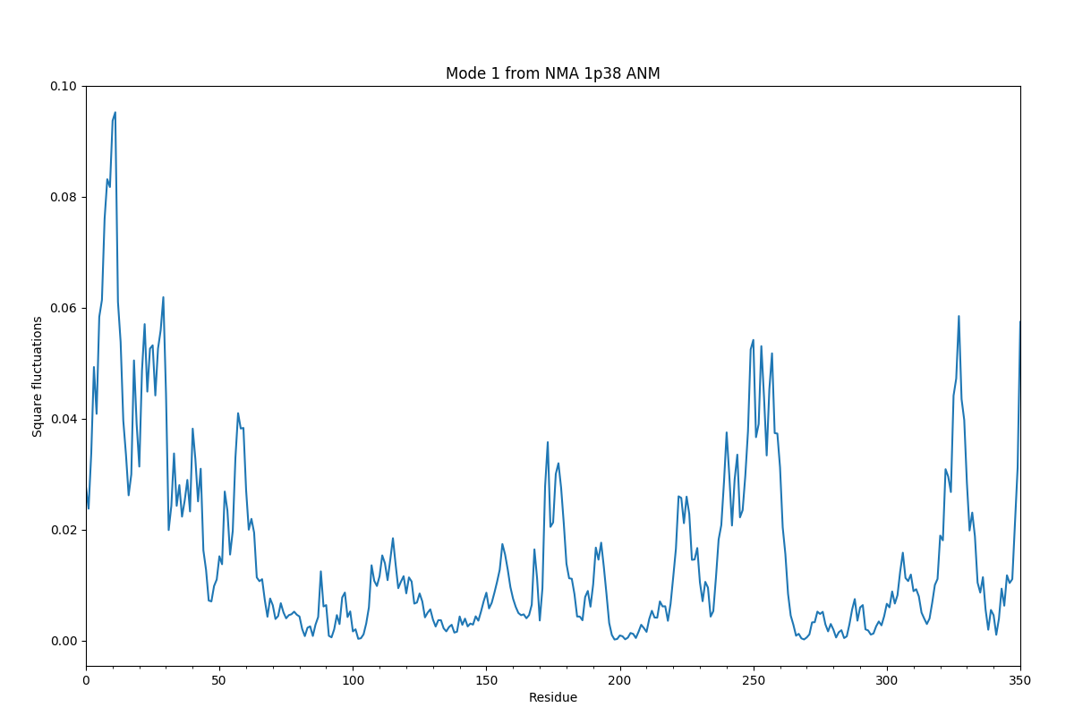
In [30]: slowmode = nma[0]
In [31]: print(slowmode.getEigval().round(2))
0.18
Plotting Data
If you have Matplotlib, you can use functions whose name start with show
to plot data:
In [32]: showSqFlucts(slowmode);
Plotting shows more plotting examples and Dynamics Analysis module documentation lists all of the plotting functions.
More Examples
For more examples and details see Elastic Network Models and Ensemble Analysis tutorials.